The manual of the MaxDiff editor: every step and control, recommended study sizes with sources, and how Choicery turns best-worst choices into individual preference scores. Worked example: the 20 pizza toppings of the Pizza (Example) study.
How to build, field, and analyse a MaxDiff (best-worst scaling) study in Choicery.
1. What Is MaxDiff?
MaxDiff (Maximum Difference Scaling), also called best-worst scaling, measures how much people prefer each item of a list. Instead of rating every item, the respondent sees a small subset of the list and picks the best and the worst item in it. Repeated over many balanced subsets and many respondents, these choices give a preference score for every item, one set of scores per person.
CBC scores product profiles made of several attributes. MaxDiff scores single items: features, claims, messages or needs, each standing on its own. If your question is "which of these things matters most?" rather than "which product would you buy?", MaxDiff is the tool.
The Pizza study used throughout this guide
The Pizza (Example) study scores 20 pizza toppings: Pepperoni, Mushrooms, Extra mozzarella, Fresh basil, Ham, Pineapple, Black olives, Red onions, Bell peppers, Italian sausage, Bacon, Spinach, Sun-dried tomatoes, Anchovies, Jalapeños, Prosciutto, Artichoke hearts, Grilled chicken, Salami and Arugula. Each task shows 4 toppings and asks: "Below are different pizza toppings. Considering your own taste, which one would you MOST like on your pizza and which one would you LEAST like?"
Why best-worst instead of a rating scale?
Ratings pile up at the top (almost everything looks "important"), and people use the scale differently: some rate everything high, others everything low. A forced best-worst choice removes both problems. The respondent must trade items off against each other, which spreads them out, and because nobody states a number, scale-use bias disappears (Orme, 2020, ch. 12.8).
What you get out of it
Individual preference scores for every item, one set per respondent.
Relative Preference, a ratio scale that sums to 100 percent: an item at 10 percent is twice as preferred as an item at 5 percent.
A rank order of the whole list.
Follow-up tools: segmentation (Latent Class) and TURF in the MaxDiff Simulation.
2. When to Use It (and When Not)
MaxDiff is the right default when you want to prioritise a list of single items and care about their order and the gaps between them.
Situation
Use
Prioritise a list of single items (features, claims, needs)
MaxDiff
You also need to know whether items are wanted at all
Anchored MaxDiff
Choose one product from multi-attribute profiles
CBC Traditional
You only need a quick rough rating and accept scale-use bias
Rating scale item
Relative, not absolute
MaxDiff scores are relative within the list: the best item wins even if respondents dislike the whole list. When you need to know whether each item is genuinely wanted, add a calibration step with Anchored MaxDiff.
3. Opening the Editor
The editor is the MaxDiff Configuration page. You reach it from the Survey Flow:
1
New block: in the Add Item panel on the right of the Survey Flow, open the section Conjoint and click or drag MaxDiff into the flow. The new block gets a free default task name (maxdiff_task, or a numbered variant if that name is taken).
2
Existing block: click Edit (gear icon) on the MaxDiff card in the flow, or click the row in the list view. A project can hold several MaxDiff blocks; each block has its own items, settings and design.
The left rail
The rail of the page has four sections:
Setup: General (opens first), Attributes (the item list), Layout.
Templates: Templates.
Output: Generate, Preview.
Help: MaxDiff Guide opens this guide in a new tab.
Only two things are required before fielding: the item list and a generated design. The Task Name and question are pre-filled. Layout and Templates are optional.
What saves automatically and what needs Save changes
Step
How it is saved
General
Manually with Save changes at the top right. The status pill reads Saved, Unsaved changes or Saving.... Leaving the page with unsaved changes asks for confirmation. A design cannot be generated while General has unsaved changes ("Save General Settings before generating the design.").
Attributes
Automatically, about 0.8 seconds after you stop typing (Autosaved, Saving..., Save failed, or Resolve duplicate attributes when a duplicate blocks the save).
Layout
Manually with its own Save changes button.
Templates, Generate
Act immediately when you click Save, Apply or Generate Design.
The two locks
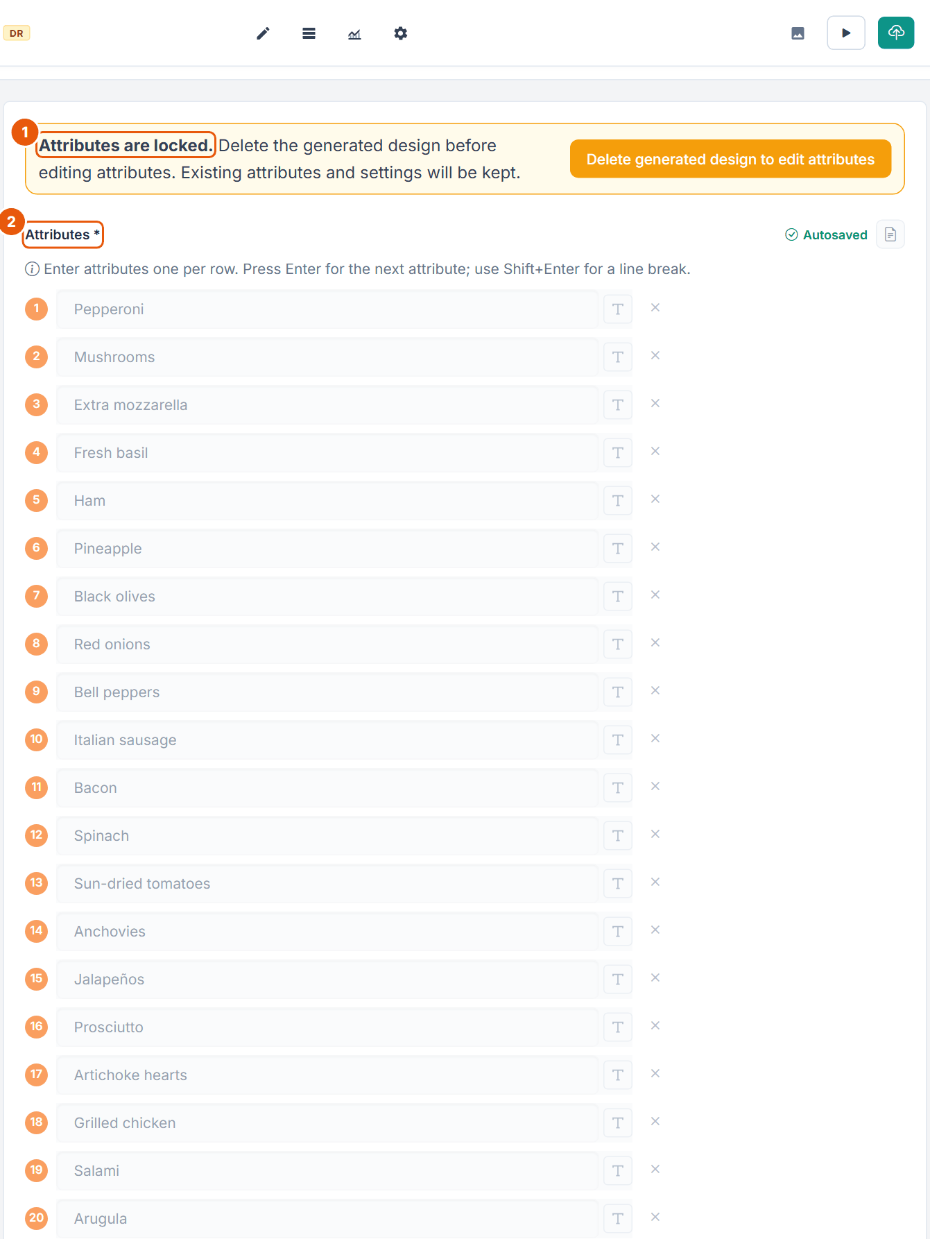
Item list locked once a design exists. The Attributes step shows "Attributes are locked. Delete the generated design before editing attributes. Existing attributes and settings will be kept." with the button Delete generated design to edit attributes (Figure 2). Deleting the design keeps the items and settings; you then generate again.
Whole design locked once responses exist. A banner "Design locked - responses already collected" names the number of active and trashed responses and explains: "To modify the design, open Data → Bin and permanently delete all responses first. To preserve them, duplicate the project before making changes. Preview, downloads, and design diagnostics remain available while the design is locked." All controls on General, Attributes, Layout, Templates and Generate are then disabled.
If the current item list and the generated design no longer match (for example after restoring an older version), a Design Warning at the top of the page says so, for example "Design is missing N item(s) from your current configuration. Please regenerate the design."
4. The Editor Step by Step
4.1 General
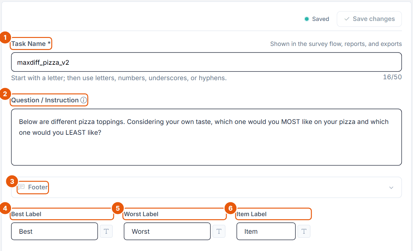
Figure 1. The General step of the Pizza MaxDiff block (task name maxdiff_pizza_v2).
No.
Control
What it does
1
Task Name *
Required. Shown in the survey flow, reports and exports; the MaxDiff export columns start with maxdiff_ plus this name. Up to 50 characters (counter on the right). Must start with a letter, then letters, numbers, underscores or hyphens.
2
Question / Instruction
The text above every task (rich text, up to 10,000 characters and 10 images). Default "Please select the best and worst item."; an emptied field falls back to this default.
3
Footer
Collapsible panel. Optional text shown below the task (placeholder "Text below the question..."), same limits as the question.
4
Best Label
Header of the best column. Default "Best". Required, up to 1,000 characters, text formatting only (no images). An empty label blocks the save: "Best label is required."
5
Worst Label
Header of the worst column. Default "Worst". Same rules.
6
Item Label
Header of the item column. Default "Item". Not shown in the Rows layout.
Write labels that match the question. The Pizza question asks what respondents would MOST and LEAST like, so labels such as "Most liked" and "Least liked" would read even more naturally than Best and Worst. The Layout step picks these labels up automatically (Column Order shows "Best first", "Worst first" with your labels).
4.2 Attributes: the item list
The step is labelled Attributes in the rail and "Attributes *" above the list, but each row is one MaxDiff item. There are no levels.
Figure 2. The item list of the Pizza block, locked because a design exists. The orange numbers 1 to 20 in front of the rows are the editor's own row numbers, not markers.
No.
Control
What it does
1
Attributes are locked.
Shown as soon as a design exists. Delete generated design to edit attributes deletes the design after a confirmation and unlocks the list; items and settings stay. With responses the design cannot be deleted (see the response lock in section 3).
2
Attributes *
The item list. Hint: "Enter attributes one per row. Press Enter for the next attribute; use Shift+Enter for a line break." Each row is a small rich-text editor (the T button opens formatting); the × removes a row (on the last row it only clears the text). To the right of the label: the autosave status and the TXT import button.
Further controls below the list (not in the figure): Add Attribute adds a row, and a counter shows "N attributes" (filled rows only).
Rule
What Choicery does
TXT import
The button ("Import from TXT file (one attribute per line)") reads a .txt file. It replaces the whole existing list and saves at once ("Imported N attributes from file."). An empty file changes nothing ("The file contains no valid entries.").
Duplicates
Two rows with the same text are blocked; capitalisation and formatting are ignored. The row shows "Duplicate of rows X, Y (capitalization and formatting are ignored)." and nothing is saved until you fix it.
Length
Up to 1,000 characters per item.
Images
At most 1 image per item (inserted through the row's editor).
Number of items
At most 100 ("MaxDiff allows at most 100 attributes"). To generate a design, you need at least 4 items: the smallest task shows 3, and at least one item must be left out. With the default 4 Items per Task, you need at least 5 items.
Free
At most 8 items per block, 4 items per task and 6 tasks. The limits apply when the list is saved and when the design is generated.
Keep every item to one clear idea at a comparable level of detail. "Extra mozzarella" and "Fresh basil" are both single toppings; an item such as "Cheese and herbs" would bundle two ideas and an item such as "Premium toppings" would be broader than the rest.
4.3 Layout
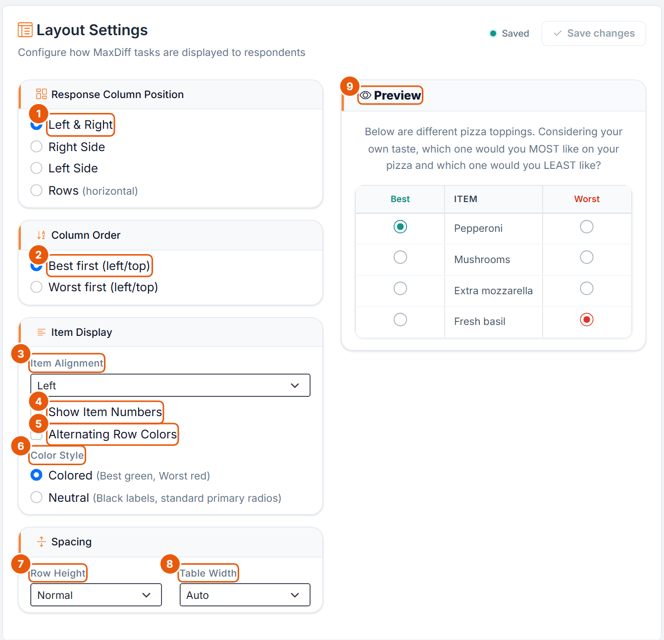
Figure 3. Layout Settings of the Pizza block with the live preview on the right.
No.
Control
What it does
1
Response Column Position
Left & Right (default: best column left, worst column right of the items), Right Side or Left Side (both answer columns on one side), Rows (horizontal: the items side by side as column headers, one row of best and one row of worst buttons below; the Item Label is not used).
2
Column Order
"Best first (left/top)" (default) or "Worst first (left/top)". The option texts use your Best and Worst labels.
3
Item Alignment
Left (default), Center or Right alignment of the item text.
4
Show Item Numbers
Numbers the items within the task. Off by default.
5
Alternating Row Colors
Shades every second row. Off by default.
6
Color Style
Colored (default: best label green, worst label red) or Neutral (black labels, standard radio buttons).
7
Row Height
Compact, Normal (default) or Spacious.
8
Table Width
Auto (default) or Custom. Custom shows Custom Width (%): 30 to 100 in steps of 5, default 80 ("30-100% of container width"). Other values are refused: "Custom width must be a whole number between 30 and 100."
9
Preview
Updates as you change settings, with the first four items and your question.
Layout changes how the task looks, not the design or the estimates. Remember to click Save changes.
4.4 Templates
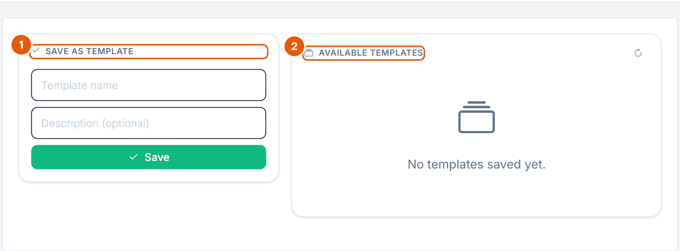
Figure 4. The Templates step, before any template has been saved.
No.
Control
What it does
1
Save as Template
Template name (required, "Enter a template name."), Description (optional), Save. Save is disabled until at least one item exists ("Define items first to save a template.").
2
Available Templates
Your saved templates with name, "N items", an expandable item list and description, and the buttons Apply, download as .txt, rename and delete. The button reloads the list.
A template stores the whole block configuration: items, question, footer, labels and layout, but not the design. Templates belong to your account and can be used in any of your projects. Apply is blocked while a design exists ("Delete the generated design before applying a template.") and asks for confirmation: "This will replace your current MaxDiff configuration, item list, and layout." The Free plan limits also apply to an applied template.
4.5 Generate
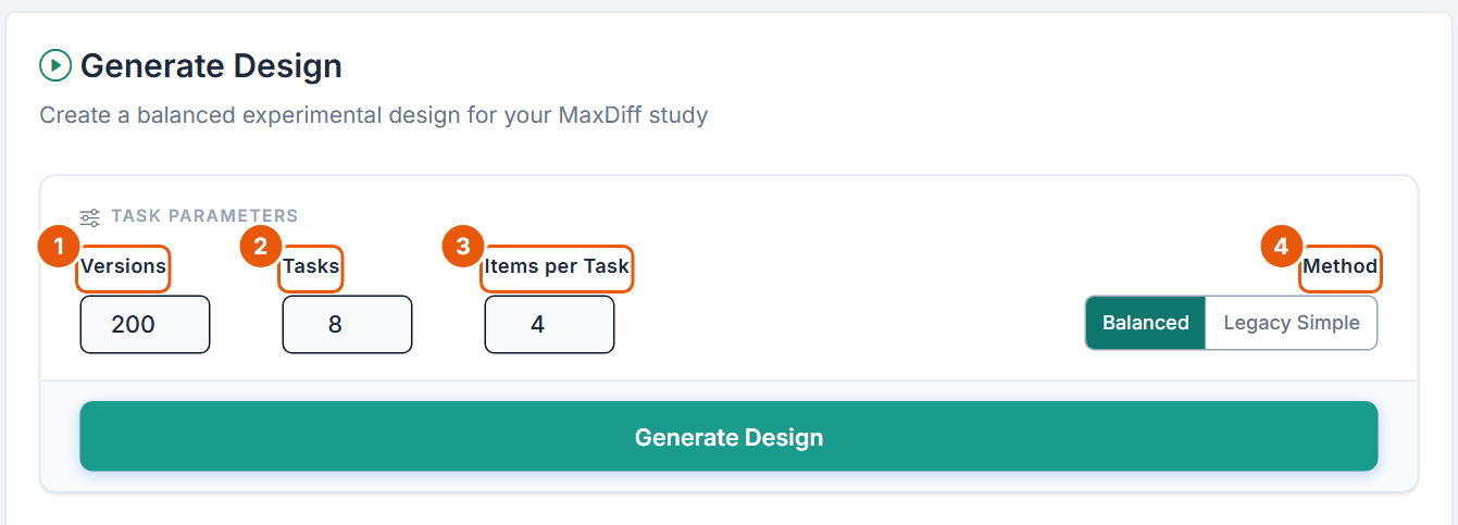
Header "Generate Design", subtitle "Create a balanced experimental design for your MaxDiff study". The editor calls one best-worst screen a Task; the literature calls it a choice set. Both words mean the same here.
Figure 5. The Task Parameters card before a design exists, with the defaults 200 versions, 8 tasks and 4 items per task.
No.
Control
What it does
1
Versions
How many different task sets (design versions) are built. Respondents are assigned to versions in rotation by participant number. Default 200 (hint "Default: 200"), allowed 1 to 300. Disabled for Legacy Simple.
2
Tasks
Best-worst tasks per respondent. Default 8 (Free plan: 6), allowed 1 to 30 (hint "Allowed: 1-30; verify respondent burden in a pretest").
3
Items per Task
Items shown in each task. Default 4, allowed 3 to 8 (hint "Allowed: 3-8; verify task comprehension in a pretest"). The field's maximum also shrinks to the number of items minus 1, because at least one item must be left out of every task. Free plan: at most 4.
4
Method
Balanced (default): "Generates multiple versions and optimizes item, pair, per-version, and position balance." Legacy Simple: "Generates one fixed task set that every respondent answers." Use Balanced unless you have a specific reason.
Generate Design is disabled while something is missing. A box above the form names the reason:
Attributes required. "Add at least 3 attributes before generating a MaxDiff design. You currently have N.", or, when Items per Task is too large: "Items per Task is set to K, so add at least K+1 attributes. At least one item must be omitted from each task; otherwise every task has the same item set."
Design parameters required. "Items per Task must be a whole number between 3 and 8."
Limited task-set variation. (warning only, generation allowed) "Each task will omit only one of the N attributes. The design is valid, but task-set variation is limited; review the diagnostics before fielding."
When you click Generate Design, Choicery checks the numbers, makes sure General is saved and saves pending item edits. If a design already exists it asks "Replace existing design?" (Replace and generate); the old design is kept as a backup in the project. If responses exist, generation is refused and a dialog points you to Data → Bin. A progress panel shows the generation with a Cancel button and ends with "Design generated successfully!".
Balanced vs Legacy Simple
Balanced builds the requested number of versions in four stages: item counts as equal as possible (exactly equal when versions × tasks × items per task is divisible by the number of items, otherwise they differ by at most one), then even pair co-occurrence, then balance within each version, then even positions on screen. For small lists, when the number of possible item subsets is at most 5,000 and the total task count is a multiple of it, Choicery uses every subset equally often instead. Details in section 14.
Legacy Simple builds one task set by rotating the least-used items. Every respondent answers the same tasks, so pair and position imbalances cannot average out across versions.
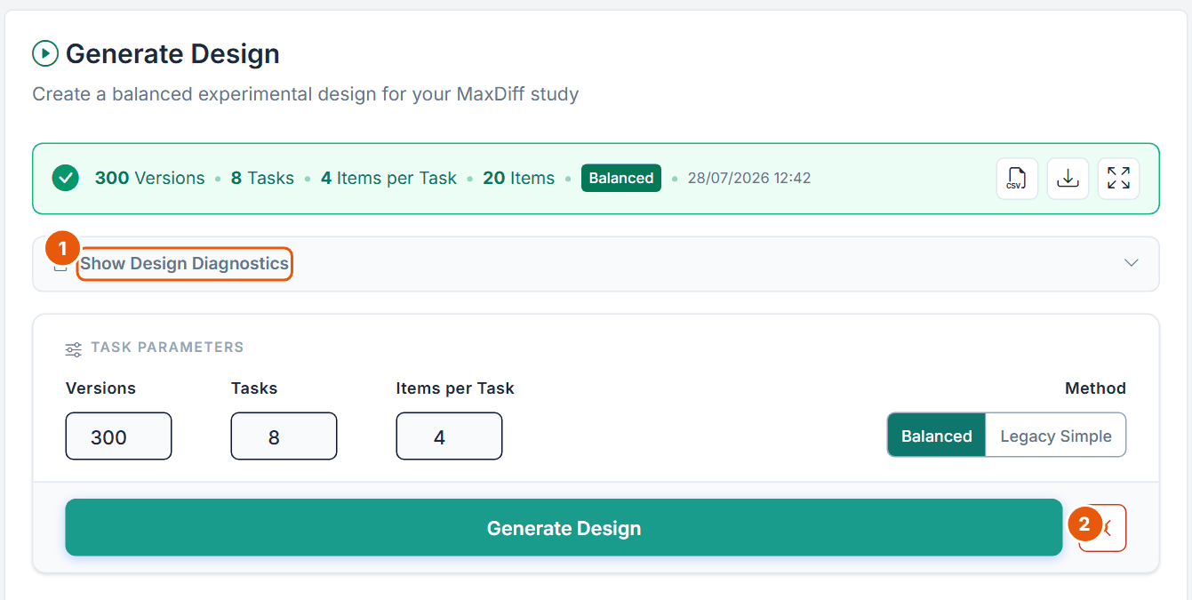
Figure 6. The Generate step after generation: the Pizza design has 300 Versions, 8 Tasks, 4 Items per Task and 20 Items.
No.
Control
What it does
1
Show Design Diagnostics
Opens the inline diagnostics summary below (section 4.6).
2
Delete design
Red button next to Generate Design. Deletes the design after the confirmation "Delete generated design?". Disabled when responses exist ("Design locked: responses already collected. Delete all responses to unlock.").
The green status bar shows the design size, the badge Balanced or Legacy Simple, the creation date and three icons: Download Design CSV, Download Diagnostics (a text report), Full Diagnostics (the full diagnostics page).
4.6 Design Diagnostics
There are two views. The inline summary under Show Design Diagnostics is a quick check. The full diagnostics page (status-bar icon Full Diagnostics) holds all measures.
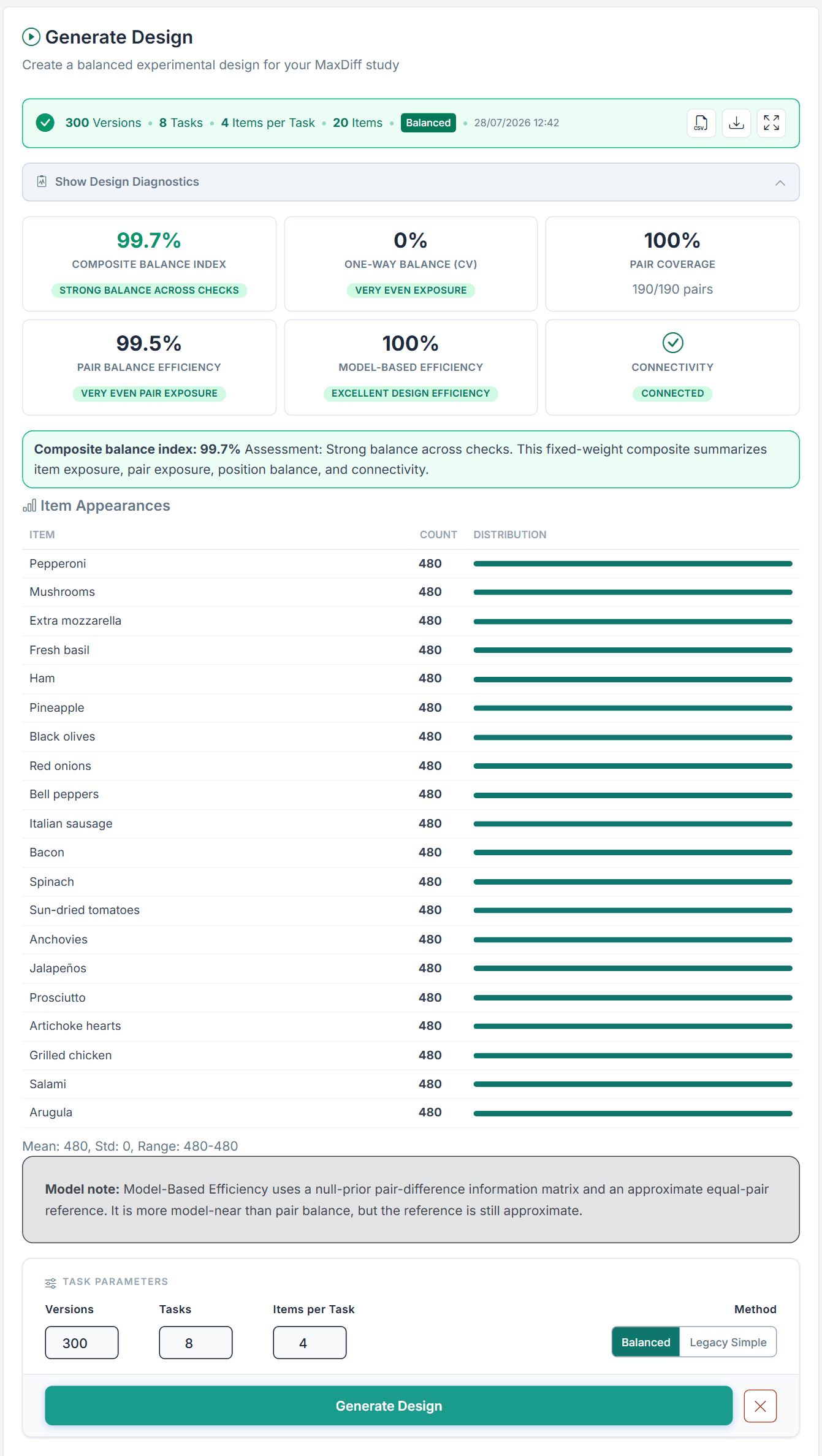
Figure 7. Inline diagnostics of the Pizza design: Composite Balance Index 99.7 percent, One-Way Balance (CV) 0 percent, Pair Coverage 100 percent (190/190 pairs), Pair Balance Efficiency 99.5 percent, Model-Based Efficiency 100 percent, Connected. Every topping appears 480 times in the whole design (300 versions × 8 tasks × 4 items / 20 items).
Measure
What it means
Target
Composite Balance Index
Fixed-weight summary of item exposure, pair exposure, position balance and connectivity.
High; read the parts below.
One-Way Balance (CV)
Coefficient of variation of the item appearance counts. Lower is better; 0 percent means every item appears equally often.
Below 5 Excellent, below 15 Good, below 30 Fair.
Pair Coverage
Share of all item pairs that appear together in at least one task (with "x/y pairs").
100 percent; a recommendation appears below 80 percent.
Pair Balance Eff.
How evenly the pairs co-occur, 100 × (1 − CV of the pair counts).
Recommendation below 70 percent.
Model-Based Eff.
Information for item differences compared with Choicery's balanced reference design. "Unavailable" means the information matrix is rank-deficient; check task validity and connectivity.
Recommendation below 70 percent.
Per-Version Exposure (full page only)
Minimum and maximum appearances of an item within one version. A zero means a version leaves an item out.
No zeros if possible.
Positional Balance (full page only)
How evenly each item is spread over the screen positions (100 minus the position-count CV).
Recommendation below 70 percent.
Connectivity
Whether all items are linked through shared tasks.
Must read Connected.
The inline summary shows the six tiles of Figure 7, recommendations, an Item Appearances table (count per item with mean, standard deviation and range) and a model note. It has no Per-Version Exposure, no Positional Balance, no pair matrix and no design information.
The full page ("MaxDiff Design Diagnostics", buttons Save PNG and Back to MaxDiff Config) adds all eight tiles with band labels, a structural alert ("Not fieldable" or "Limited task-set variation") when needed, and the sections Design Information, Model-Based Efficiency (Value, Status, Matrix Rank, Task Basis), One-Way Frequencies, Two-Way Frequencies (pair heat matrix), Positional Balance per item, and Recommendations.
What to do when a measure is weak
Follow the recommendation text on the page. For low pair coverage it says: compare regenerated candidates first; if the gap remains, weigh additional tasks against respondent burden. For model-based efficiency it notes that "this metric alone does not prescribe more tasks or versions". A disconnected design must be regenerated before fielding. Small lists with few tasks can never cover all pairs within one respondent; what matters is coverage across the whole design.
4.7 Preview
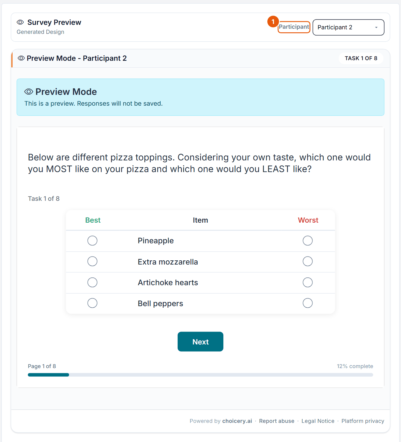
Figure 8. Preview of the generated Pizza design, Participant 2, task 1 of 8: Pineapple, Extra mozzarella, Artichoke hearts and Bell peppers.
No.
Control
What it does
1
Participant
Picks the design version to preview ("Participant 1" up to the number of versions; Legacy Simple has one). The preview uses the real survey page and steps through all tasks with Next. Answers are not saved.
Without a design, the subtitle reads "Example Preview" and Choicery shows one example task built from the first items of your list (at least two items are needed: "Define at least two items to see an example preview."). With a design it reads "Generated Design".
5. How Large Should Your Study Be?
The editor allows far more than the literature recommends. Use the table to set the four numbers; the sources and their disagreements follow.
Setting
Recommendation
Source
Choicery allows
Items in the list
Typically 8 or more. No source gives a maximum for individual-level (HB) MaxDiff.
Orme (2020), ch. 12.2, p. 119
3 to 100 (Free plan 8)
Items per task (k)
4 to 5 (the common ground of 4 to 6, 3 to 5 and 3 to 4)
Orme (2020), p. 119; Rao (2026), ch. 16.8, p. 525; Schramm & Lichters (2024), p. 2
3 to 8, default 4 (Free plan 4)
Appearances per item and respondent
About 3, so tasks = 3 × K / k (K = number of items)
Rao (2026), p. 525: 16 items, 4 per set, "with twelve choice tasks, each item would be shown three times"
follows from Tasks and Items per Task
Tasks per respondent
8 to 20; the median in business research is 12 to 13
Orme (2020), p. 119; Schramm et al. (2025), p. 11 (citing Schuster et al., 2024)
1 to 30, default 8 (Free plan 6)
Versions
Many, ideally individual designs
Schramm et al. (2025), p. 37 (300 versions, one per respondent, p. 12)
1 to 300, default 200
Respondents
No MaxDiff-specific rule in the literature reviewed
see below
no limit in the editor
Table 1. Recommended MaxDiff sizes and the Choicery limits.
Items per task and appearances
Orme (2020, p. 119) gives 4 to 6 items per set, Rao (2026, ch. 16.8, p. 525, a chapter written by Orme) 3 to 5, and Schramm and Lichters (2024, p. 2, citing Louviere et al., 2013) 3 to 4. All overlap at 4; 4 to 5 is the common ground. More items per task turn the judgment into a mini-ranking. The rule "each item about 3 times" comes from Rao's worked example; it is a rule of thumb, not a tested threshold.
The Pizza study in numbers
K = 20 toppings, k = 4 per task. For about 3 appearances you need 3 × 20 / 4 = 15 tasks. With 5 items per task it would be 3 × 20 / 5 = 12 tasks. The Pizza example uses 8 tasks, so each respondent sees 32 item slots and each topping about 1.6 times. Across all respondents the design is still perfectly balanced (480 appearances per topping, Figure 7), but individual scores lean more on the HB population model. For individual-level results, raise Tasks to 12 to 15.
tasks needed = 3 x K / k
Pizza: 3 x 20 / 4 = 15 tasks (or 3 x 20 / 5 = 12 tasks)
Free plan maximum: 3 x 8 / 4 = 6 tasks (exactly the Free plan limit)
Tasks per respondent
Orme (2020, p. 119) reports 8 to 20 sets as typical. Schramm et al. (2025, pp. 11, 35 to 37) find that the median of 12 to 13 tasks is too few for the best prediction with indirect or status-quo anchors, while direct anchoring reaches its best with fewer tasks; unlike CBC, they found no harmful fatigue effect over 16 tasks. In the same study the median time per task fell from about 19 to 30 seconds for the first task to about 9 to 10 seconds later (four items, pp. 26 to 27). MaxDiff takes about three times as long as a rating battery of the same items (Orme, 2020, ch. 12.5, p. 126).
Many items: sparse and bandit designs
Choicery's limits (at most 30 tasks and 8 items per task, so 240 item slots per respondent) reach about 3 appearances per item for up to 80 items with 8 per task, 50 items with 5 per task, or 40 items with 4 per task. Beyond that each respondent sees each item fewer than three times. For long lists Orme (2020, ch. 12.7, pp. 128 to 129) describes two approaches:
Sparse MaxDiff: each item seen about once per respondent, for example 80 items in 20 sets of 4, with about 1,000 respondents, analysed in aggregate (pooled logit or counts) rather than per person. You can build such a design with the Balanced method (80 items, 4 per task, 20 tasks). Choicery estimates MaxDiff with individual-level HB, so read individual scores from a sparse design with care; the averages are the robust output.
Bandit MaxDiff: an adaptive design that shows the currently strongest items more often, for 80 to 500 items; with 120 or more items it is reported to be 3 to 4 times as efficient as Sparse at finding the top items (250 to 333 respondents instead of 1,000; Fairchild, Orme & Schwartz, 2015, cited in Orme, 2020). Choicery has no adaptive (bandit) MaxDiff design.
Versions
Schramm et al. (2025, pp. 12, 37) used 300 versions, one per respondent, and recommend individualised designs so that HB can recover preferences even from few tasks. Choicery's default is 200 and the maximum 300. Respondents beyond the number of versions reuse versions in rotation, which does not harm the design.
Sample size
The sample size for standard MaxDiff is not settled in the literature reviewed for this guide: none of the sources gives a rule. As orientation, the two anchoring experiments used 448 respondents in a 2 × 2 design (Schramm & Lichters, 2024) and 1,468 respondents (Schramm et al., 2025), and Orme (2020) suggests about 1,000 for Sparse MaxDiff. If you report subgroups, plan each subgroup as its own sample. CBC rules of thumb (at least 300 respondents, or 200 per reported subgroup; Orme & Chrzan, 2017, ch. 8) are a conservative orientation, not a MaxDiff rule.
6. The Best-Worst Task the Respondent Sees
Each task shows the question, a counter ("Task 1 of 8"), the table in the chosen layout, the footer and a Next button (Figure 8). The respondent marks exactly one item as best and one as worst. The Back button is disabled within MaxDiff tasks. Missing answers are reported with 'Please select one "Best" item and one "Worst" item.' (or only the missing one), and the same item in both columns with 'The same item cannot be selected for both "Best" and "Worst".' The messages use your labels.
One best plus one worst says more than a single pick: the best item beats the other three, and the worst item loses to the other three. A four-item task therefore gives five of its six pairwise comparisons at once.
How the answer is stored
Each shown item becomes one row. The best item is coded 1, the worst -1, the others 0. This is the schema of the long-format export and of the MaxDiff file import. Suppose Participant 2 in task 1 of Figure 8 picks Extra mozzarella (item 3) as best and Artichoke hearts (item 17) as worst:
ID
Set
Position
Item
Response
2
1
1
6
0
2
1
2
3
1
2
1
3
17
-1
2
1
4
9
0
Table 2. Long-format rows for one task (columns ID, Set, Position, Item, Response). Items 6, 3, 17, 9 are Pineapple, Extra mozzarella, Artichoke hearts and Bell peppers.
The file has respondents × tasks × items per task rows. A companion attributes file maps item numbers to labels. Both are in the ZIP behind MaxDiff Responses (Long Format) on the Export step of the analysis.
7. Estimating Scores with Hierarchical Bayes
After fieldwork, open the analysis and stay on the Preference Analysis (HB) tab. The card MaxDiff Preference Estimation (HB) estimates a full set of item scores for every respondent and borrows strength from the whole sample.
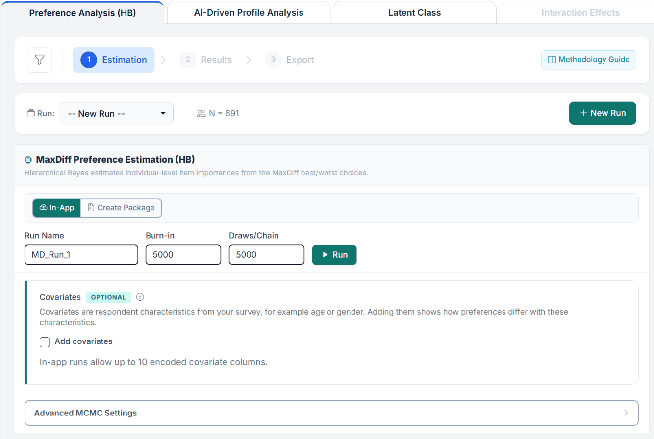
Figure 9. The Estimation step of the Pizza MaxDiff for a new run (N = 691): Run Name, Burn-in and Draws/Chain with their defaults.
Run Name (suggested MD_Run_1), Burn-in and Draws/Chain (both 5,000 by default).
In-App runs on the server (at most 2 chains, a shared total of 100,000 burn-in plus draws per chain, about two hours wall time). Create Package exports a Julia replication package for your own machine (up to 20 chains, 500,000 burn-in and 500,000 draws per chain) whose results you import again.
Covariates (optional): respondent characteristics that shift the item scores. The panel states whether in-app runs accept covariates and how many encoded columns.
Advanced MCMC Settings: Seed (42), Chains (2), Parallel (package only), Individual R-hat, a random holdout task, a validation split, Variance Adj. (default 4.0, 1.0 to 10.0; the main prior setting for MaxDiff) and Prior σ² (default 1.0, 0.1 to 5.0).
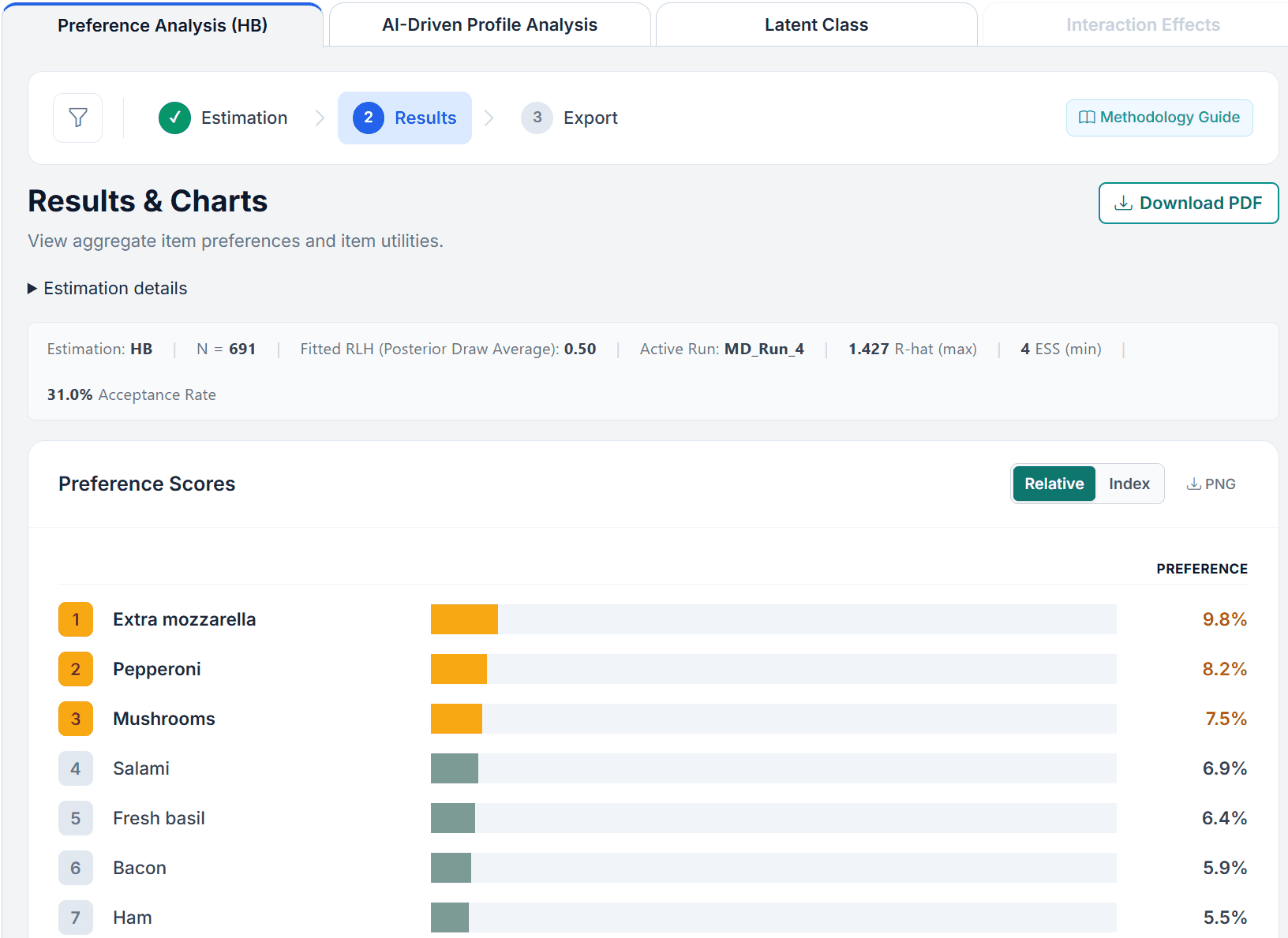
Figure 10. Results of the Pizza run MD_Run_4 (50,000 burn-in, 5,000 draws per chain): meta bar and Preference Scores in the Relative view. Extra mozzarella leads with 9.8 percent, followed by Pepperoni (8.2) and Mushrooms (7.5). The run is too short and not converged (R-hat 1.427, ESS 4), which shows what to look for before reporting.
Convergence first
The meta bar shows Estimation, N, Fitted RLH (Posterior Draw Average), Active Run, R-hat (max), ESS (min) and the Acceptance Rate. R-hat below 1.1 is acceptable and below 1.05 good; it needs at least 2 chains. RLH is the geometric mean of the predicted probabilities of the observed picks; chance is 1 / items per task (0.25 with 4 items). The Pizza run in Figure 10 has RLH 0.50, well above chance, but R-hat 1.427 and ESS 4. It kept only 5,000 draws per chain (1,000 after thinning), far too few for 20 items: the worst values belong to the variance terms (Sigma), above all the one of Anchovies, an item respondents almost always picked as worst (0.4 percent). Such terms mix slowly, so they need many more draws. The same data run again with 50,000 draws per chain (replication package, same seed) reached R-hat (max) 1.058 with no parameter above 1.1, and the item means reached an ESS of at least 125; only a few variance terms stayed below 100. Increase Draws/Chain (and Burn-in) until R-hat (max) is below 1.1 and ESS (min) is well above 100 before you report. The acceptance rate is tuned toward about 30 percent.
The score scales
The Relative and Index buttons in the Preference Scores header switch between two scales with the same ranking:
Relative Preference: sums to 100 percent and is ratio-scaled. Extra mozzarella (9.8 percent) is about twice as preferred as Bell peppers (5.0 percent).
Preference Index: Relative Preference times the number of items, so the average item is 100. With 20 toppings, Extra mozzarella's 9.8 percent becomes an index of about 196. Use it to compare studies with different list lengths.
The Excel workbook MaxDiff Results (Excel) on the Export step adds the sheets Worst-Zero Interval Scale (each respondent's lowest item at 0) and Zero-Centered Raw Scores (logit scale, mean 0, for statistical analysis), next to Relative Preference, Preference Index, Preference Share and a Settings Summary whose SCALE NOTES define every scale.
Holdout validation and covariate effects
With a random holdout task, the results add Holdout Validation (Best, Worst and Average hit rates against chance). With covariates, Covariate Effects lists the mean shift per covariate and item in percentage points ("Mean (pp)", or the utility scale), P(+), P(−) and a 95 percent credible interval, followed by Share Explained by Covariates. Numeric covariates are z-standardised; categorical ones are shown against their reference level.
Next step: MaxDiff Simulation
The item scores feed the MaxDiff Simulation (in the header navigation), which answers reach questions: which small set of toppings appeals to the most people, and where extra items stop adding reach. See the MaxDiff Simulation guide.
9. Best Practices & Pitfalls
Do
Keep every item to one clear idea at a comparable level of detail.
Show 4 to 5 items per task and plan about 3 × K / k tasks so each item is seen about three times.
Use the Balanced method with many versions, and check Connectivity and Pair Coverage before fielding.
Walk through several participants in Preview before you go live.
Check R-hat and RLH (chance is 1 / items per task) before reporting anything.
Use Anchored MaxDiff when you need to know whether items are wanted at all.
Do not
Do not mix broad and narrow items; the broad ones win for the wrong reason.
Do not make one item much longer or more vivid than the rest. MaxDiff has no levels, so the CBC number-of-levels effect does not apply, but presentation effects do.
Do not overload a task; more than six items turns each judgment into a mini-ranking.
Do not import a TXT file into a list you have already edited unless you want to replace it.
Do not read Relative Preference as "wanted or not wanted"; it is relative within the list.
Part II
Theoretical Background
Random utility, the best-worst logit choice rule, and Hierarchical Bayes estimation.
10. Key Definitions
Item
One element of the list being scored (a feature, claim or need). The MaxDiff editor lists items on the Attributes step.
Task (choice set)
A subset of the list shown together on one screen.
Best-worst response
The pair of picks in a task: one item best (+1), one worst (−1), the rest 0.
MaxDiff (best-worst scaling case 1)
The design in which the alternatives are single items and the respondent selects the best and the worst in each set. Case 2 asks for the best and worst level within one profile, case 3 for the best and worst profile.
Version
One complete task sequence of the design. Respondents are assigned to versions in rotation.
Hierarchical Bayes (HB)
An estimation method that models each respondent's item scores as drawn from a population distribution, so individual estimates borrow strength from the group.
Relative Preference (probability scale)
The ratio-scaled report of item scores that sums to 100 per respondent.
Preference Share
A softmax share: exp(u) divided by the sum of exp(u) over all items, times 100. Also sums to 100 but is much steeper than Relative Preference.
Preference Index
The probability scale multiplied by the number of items, so the average item is 100.
RLH (root likelihood)
Geometric mean of the predicted probabilities of the choices a respondent made. Chance is one over the number of items per task.
11. The Random Utility Model & the Best-Worst Logit
MaxDiff rests on random utility theory (McFadden, 1974; Marley & Louviere, 2005). Respondent h assigns to item i a utility that is a systematic score plus a random error:
Uhi = βhi + εhi
Utility of item i for respondent h; βhi is the respondent's score for the item.
With independent extreme-value (Gumbel) errors, the probability of picking item i as best from the shown set S is a multinomial logit:
P(best = i | S) = exp(βi) / Σk in S exp(βk)
Best choice: the highest-utility item wins among the items shown.
The worst pick is the same rule on the negated scale:
P(worst = j | S) = exp(−βj) / Σk in S exp(−βk)
Worst choice: best = max(U), worst = max(−U). The design matrix for the worst pick is negated.
Choicery stacks the best and worst responses into one estimation with the worst pick's design negated (Orme, 2020). This is the logit family that CBC uses; only the alternatives differ, and each task contributes a best and a worst observation.
12. Hierarchical Bayes Estimation
HB estimates individual item scores and a population distribution that ties them together (Lenk, DeSarbo, Green, & Young, 1996; Rossi, Allenby, & McCulloch, 2005):
Individual item scores are drawn from a population normal. The population mean has a weak normal prior with variance Prior σ² (default 1.0). The covariance has an Inverse-Wishart prior whose expected value is Variance Adj. times a fixed effects-coding matrix with (K−1)/K on the diagonal and −1/K off the diagonal (K = number of items), so every item, including the last one, gets the same prior variance and Variance Adj. sets how much heterogeneity the prior expects.
The sampler alternates three steps per iteration: a Random-Walk Metropolis update of each respondent's βh (proposals shaped by the current Σ), a Gibbs draw of μ, and a Gibbs draw of Σ. The best-worst likelihood from section 11 enters at the Metropolis step. Convergence checks and settings are covered in the HB guide.
Why HB instead of one aggregate model?
If half the market loves Anchovies and half hates them, an aggregate model makes them look average and describes nobody. HB recovers each person's own scores, which is what segmentation and TURF need.
Aggregate model: one beta per item for everyone.
HB: one beta_h per respondent, drawn from MVN(mu, Sigma).
TURF over a niche segment only works with the individual beta_h.
13. Effects Coding & the Score Scales
Items enter the model through effects coding: for K items, K−1 columns are estimated and the last item is the negative sum of the others, so the raw scores sum to zero:
Effects coding. The reference item is the negative sum, so Σ scores = 0 across the list.
These are the Zero-Centered Raw Scores (logit scale, interval-scaled). Three rescalings make them easier to read:
Worst-Zeroi = βi − mink βk
Worst-Zero Interval Scale: each respondent's lowest score becomes 0.
ri = 100 × exp(βi) / ( exp(βi) + a − 1 ) Probabilityi = 100 × ri / Σk rk
Relative Preference. Each item is turned into the probability of being picked from a hypothetical set of a items (a = items per task) where all other items are average, then normalised to sum to 100.
Indexi = K × Probabilityi
Preference Index: the average item lands at 100 regardless of study size.
The exponential step makes Relative Preference a ratio scale; the Index inherits that property. The Zero-Centered and Worst-Zero scales are interval scales: differences are meaningful, ratios are not.
RLH = ( Πt pt )1 / T
Geometric mean over the T best and worst observations. Chance is 1 / items per task (0.25 for four per task).
14. Experimental Design
A good MaxDiff design has frequency balance (each item about equally often), pairwise balance (each pair about equally often together) and positional balance (no item always at the top or bottom) (Orme, 2020, ch. 12.2 to 12.3; Rao, 2026, ch. 16.8). Counting analysis needs near-perfect balance; HB is more forgiving.
Choicery's Balanced generator works in four stages, each preserving the earlier ones:
Item counts: exactly equal when versions × tasks × items per task is divisible by the number of items, otherwise differing by at most one.
Pair balance: swaps items between tasks so pairs co-occur as evenly as possible.
Version balance: arranges tasks so each version is balanced on its own.
Position balance: swaps items within a task so no item keeps the same row.
When the number of possible item subsets is at most 5,000 and the total number of tasks (versions × tasks) is a multiple of it, Choicery uses every subset equally often instead, which gives perfect item and pair balance by construction, and then runs only the version and position stages. The Design Diagnostics report the achieved values for each design.
Why a subset per task, not the whole list?
Showing all items at once turns the task into a full ranking, which tires respondents. Showing a handful keeps each judgment quick, while the design links the subsets so that, across tasks and versions, every item is compared directly or indirectly with every other. Prohibitions hurt MaxDiff much less than CBC but make counting analysis inaccurate (Orme, 2020, ch. 12.4).
15. References
Finn, A., & Louviere, J. J. (1992). Determining the appropriate response to evidence of public concern: The case of food safety. Journal of Public Policy & Marketing, 11(2), 12-25.
Lenk, P. J., DeSarbo, W. S., Green, P. E., & Young, M. R. (1996). Hierarchical Bayes conjoint analysis: Recovery of partworth heterogeneity from reduced experimental designs. Marketing Science, 15(2), 173-191.
Louviere, J. J., Flynn, T. N., & Marley, A. A. J. (2015). Best-worst scaling: Theory, methods and applications. Cambridge: Cambridge University Press.
Louviere, J. J., & Woodworth, G. (1983). Design and analysis of simulated consumer choice or allocation experiments: An approach based on aggregate data. Journal of Marketing Research, 20(4), 350-367.
Marley, A. A. J., & Louviere, J. J. (2005). Some probabilistic models of best, worst, and best-worst choices. Journal of Mathematical Psychology, 49(6), 464-480.
McFadden, D. (1974). Conditional logit analysis of qualitative choice behavior. In P. Zarembka (Ed.), Frontiers in econometrics (pp. 105-142). New York: Academic Press.
Orme, B. K. (2020). Getting started with conjoint analysis: Strategies for product design and pricing research (4th ed.). Manhattan Beach, CA: Research Publishers.
Orme, B. K., & Chrzan, K. (2017). Becoming an expert in conjoint analysis: Choice modeling for pros. Orem, UT: Sawtooth Software.
Rao, V. R. (2026). Applied conjoint analysis: From product and service design to market and pricing strategies (2nd ed.). Springer. (Chapter 16 is written by B. Orme.)
Rossi, P. E., Allenby, G. M., & McCulloch, R. (2005). Bayesian statistics and marketing. Chichester: John Wiley & Sons.
Schramm, J. B., & Lichters, M. (2024). Incentive alignment in anchored MaxDiff yields superior predictive validity. Marketing Letters, 36(1), 1-16 (2025 issue). https://doi.org/10.1007/s11002-023-09714-2
Schramm, J. B., Lichters, M., & Guhl, D. (2025). Anchoring methods for MaxDiff and their predictive validity in product choice. SSRN preprint 5674983, not peer reviewed.
Train, K. E. (2009). Discrete choice methods with simulation (2nd ed.). Cambridge: Cambridge University Press.