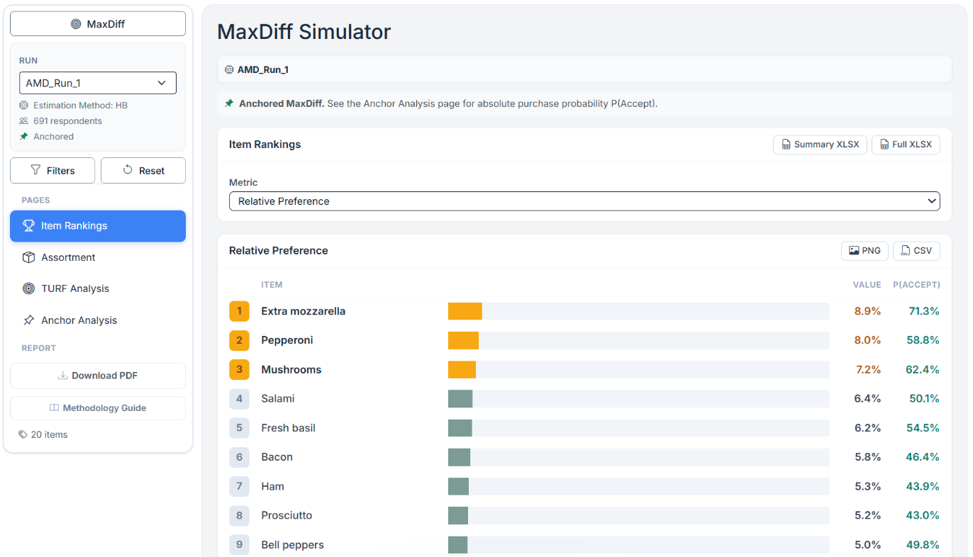
Turning MaxDiff preference scores into item rankings, share of choice, optimal assortments (TURF), and absolute purchase probabilities. A complete reference to every page in the Choicery MaxDiff Simulation workspace.
How to use the MaxDiff Simulation page in Choicery, page by page, in the order you meet them.
A MaxDiff (best-worst scaling) study asks people which item they like most and least, again and again, across many small sets. After estimation (Hierarchical Bayes), every respondent ends up with an individual preference score for each item. On its own, that is just a pile of numbers. MaxDiff Simulation is the page where you turn those scores into decisions.
The page is organised as a short sequence of analyses, and you meet them in this order:
A car manufacturer ran a MaxDiff study on eight features and now wants to know which features to feature prominently. We will use this study in every section:
| Item # | MaxDiff item (feature) |
|---|---|
| 1 | Safety Rating |
| 2 | Fuel Efficiency |
| 3 | Interior Space |
| 4 | Design |
| 5 | Resale Value |
| 6 | Technology Package |
| 7 | Warranty |
| 8 | Brand Reputation |
The MaxDiff Simulation page is a consumer of analysis results, not an estimator. Before it shows anything, two things must already exist.
A MaxDiff or Anchored MaxDiff task. TURF is only available for MaxDiff studies. If the project has no MaxDiff task, the page shows the message "This project contains no MaxDiff or Anchored MaxDiff tasks. TURF analysis is only available for MaxDiff studies."
A completed Preference Analysis (HB) run for that task. TURF needs individual-level utilities, which come from the Hierarchical Bayes estimation. If no completed run exists, the page shows "No Completed Run for This Task" with a button Go to Preference Analysis. Run HB first, then return.
The page has a left sidebar for choosing what to analyse and a main area with one page per analysis. The sidebar is always visible.
The Run dropdown (a standard <select> control) lists every completed MaxDiff
run in the project. Each option carries its own task, so picking a run from a different task (for example
switching between a normal and an Anchored MaxDiff study) switches the task automatically. Choicery detects
whether the selected run is anchored and shows the Anchor Analysis page accordingly.
The Filters button restricts every analysis on the page to a subset of respondents, defined by their answers to other survey questions (for example "women under 35" or "premium buyers"). When a filter is active, rankings, share-of-choice, and TURF reach recompute on that subset. The Anchor Analysis calibration cards remain a full-run diagnostic and say so explicitly. This is the same shared segment filter used by the Market Simulator.
The main area has up to four pages, selected from the Pages list:
| Page | What it answers |
|---|---|
| Item Rankings | How do the items rank, under five different definitions of "preferred"? |
| Assortment | If only these items were on offer, what share would each win? |
| TURF Analysis | Which set of K items reaches the most respondents? |
| Anchor Analysis | (Anchored MaxDiff only) What is each item's absolute purchase probability? |
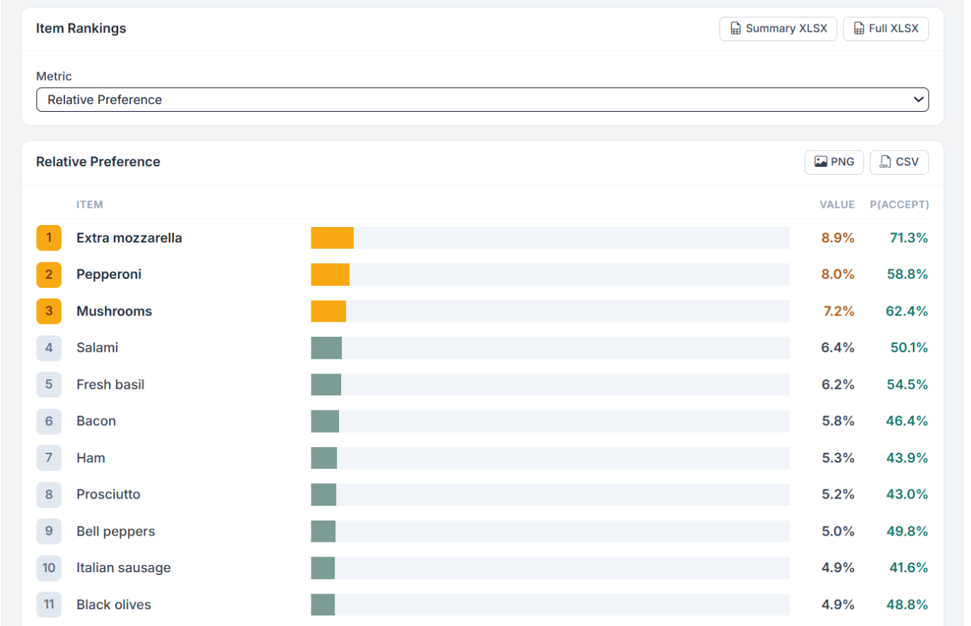
The Item Rankings page ranks all MaxDiff items. A single Metric dropdown switches between five views of the same individual utilities. Each metric answers a slightly different question, so they can produce different orderings, which is exactly why all five are offered.
| Metric | What it measures | Sums to |
|---|---|---|
| Relative Preference | Mean individual preference share: each respondent's MaxDiff utilities are converted to a 100% share across all items, then averaged. The default view. | 100% across items |
| First Choice | Share of respondents whose single highest-utility item is this item. Exact ties split equally. | 100% across items |
| Softmax Preference Share (%) | The softmax share exp(u) / Σ exp(u) averaged over respondents. | 100% across items |
| Shapley Contribution | Each item's fair share of total TURF reach, averaged across portfolios (see Section 13). | 100% across items |
| Rank Comparison | A table that keeps the Relative Preference order and shows each item's rank under all the other methods side by side. | n/a |
100 / 8 = 12.5% across each. So
anything above 12.5% is an above-average item and anything below is below-average. In Figure 3,
Safety Rating at 22.4% is nearly twice the random baseline; Design at 7.6% is well below it.
First Choice is "winner takes all" per respondent, so it rewards items that are somebody's absolute favourite, even a polarising item that many others rank last. Relative Preference is a smoother average. An item that is nobody's number one but everybody's solid number two can rank higher on Relative Preference than on First Choice. Reading both protects you from a single misleading view.
The Assortment page answers: "If the only options were the ones I tick, what share would each capture?" Tick the items in the Select Assortment card, click Simulate, and Choicery computes a share of choice on the individual utilities and averages across respondents. At least two items must be ticked; with fewer, the page answers "Select at least 2 items."
Use this page to compare line-ups directly: "if we only promoted Safety, Fuel Efficiency, and Design, Safety takes almost half the attention." It is the MaxDiff cousin of CBC market simulation, but on items rather than full product profiles.
This is the heart of the page. You set up to four controls, click Run TURF, and Choicery searches for the item sets that reach the most respondents.

| Setting | Meaning | Default |
|---|---|---|
| Assortment Size | How many items go in the set you are optimising (the K in "best K items"). Maximum is the number of items in the study. | 3 |
| Ladder Size | How far the greedy ladder builds (Section 12). The ladder shows the best 1 item, then 2, up to this size. | 5 |
| Reach Definition | What counts as "this item is acceptable to this respondent". See below. | Item is in respondent's top-K |
| K (top items) | Only used when the reach definition is "top-K": an item counts if it is in the respondent's personal top-K. K is capped one below the number of items, so a set can never reach everyone by definition alone. | Top quartile of the item list, at most 5 (see below) |
How the default K is chosen. When you do not set K yourself, Choicery uses the top quartile of the item list, capped at 5: K = max(1, min(5, ceil(number of items / 4))). In practice that is 6 items → 2, 8 → 2, 10 → 3, 12 → 3, 16 → 4, 20 or more items → 5. A fixed default of 5 would make reach trivially high in short lists: with "top 5 of 6" almost every item reaches almost every respondent, so every assortment looks equally good. Tying K to the list length keeps "reached" meaningful across studies of different sizes. A K you type in is used as entered; it is only limited to one below the number of items, and the results card says so when that happens.
There is no execution-mode setting. A search that does not fit the interactive work budget (Section 12) is handed to the analysis worker automatically when a worker is available, and the results appear when it finishes (the page waits up to 15 minutes). Without a worker, Choicery returns a message asking for a respondent segment, a smaller assortment or fewer items.
The Reach Definition is the most important choice on this page. It decides how strict "acceptable" is, and it can completely change the answer. Choicery offers five definitions for every MaxDiff run, plus two more on anchored runs:
| Option (verbatim) | An item reaches a respondent when... | Strictness |
|---|---|---|
| Item is in respondent's top-K | ...the item is among that respondent's top-K items by utility (K is the control above). | Adjustable (default) |
| Weighted by probability | ...the selected items' exponentiated utilities are combined into one portfolio probability (see Section 11). The reported "Reach %" is then a mean probability, not a head count, and it does not reach 100% even for the full item set; the level depends on the number of items per MaxDiff set (see the note in Section 11). | Balanced |
| First Choice (top item; ties split) | ...the portfolio contains the respondent's highest-utility item. Exact ties split one unit across the tied items. | Strict |
| Item is in respondent's top half | ...the item is above the respondent's median utility. | Lenient |
| Item is above respondent's mean (lenient) | ...the item is above the respondent's mean utility (which for MaxDiff is 100/n items). | Very lenient |
| Calibration "Yes" answers (raw) | ...the respondent answered "Yes" to the item on the calibration screen. Only shown for Anchored MaxDiff. | Real acceptance |
| Utility above anchor (model-based) | ...the item's estimated utility is above the respondent's anchor threshold from the HB model. Only shown for Anchored MaxDiff runs that carry anchor thresholds. | Model-based acceptance |
Before you run anything the results card is headed TURF Results. After Run TURF it is replaced by a card headed Optimal K-Item Assortment (with K the assortment size you chose), and the table inside it carries the sub-heading Top N Combinations, or Best Combination when only one is returned. It lists the best item combinations, ranked by reach. The best row is highlighted. Each combination shows its item IDs (the bracketed numbers), the item names, its reach and its frequency. Under the Weighted by probability reach definition the table changes its two right-hand columns: the ID column is headed Portfolio, and instead of Freq. you get Total, the summed portfolio probability across respondents.
| # | IDs | Items | Reach | Freq. |
|---|---|---|---|---|
| 1 | [1][2][4] | Safety Rating · Fuel Efficiency · Design | 88.1% | 1.7 |
| 2 | [1][2][6] | Safety Rating · Fuel Efficiency · Technology Package | 86.5% | 1.8 |
| 3 | [1][2][5] | Safety Rating · Fuel Efficiency · Resale Value | 85.9% | 2.0 |
Alongside the best combinations, Choicery builds a ladder up to your Ladder Size. It is a greedy build: start with the single item that reaches the most people, then add the item that adds the most new reach, and so on. Each row names the added item, its Gain (the marginal reach that item adds on top of the previous step), the Cumulative Reach of everything selected so far, and a Status column that reads "Adds reach" or, once reach has plateaued, "Redundancy only". The cumulative reach bar shows how quickly you saturate.
Reach often plateaus before the ladder is finished: at some point no remaining item can raise it any further. The ladder does not stop there. It keeps building to the size you asked for and marks those steps Redundancy only, with a Gain of +0.0%. At those steps, remaining candidates are ranked by Frequency instead of additional reach. With a binary reach rule, Frequency is the average number of selected items that pass each respondent's reach criterion; under Weighted by probability, it is the average summed item-probability mass. A candidate can tie on both measures, so adding it does not necessarily increase Frequency. A note under the table names the plateau value. Note that the plateau is not always 100%: with a binary reach rule, part of the sample can be unreachable by any item in the pool.
| Size | ID | Added Item | Gain | Cumulative Reach | Status |
|---|---|---|---|---|---|
| 1 | [1] | Safety Rating | +62.0% | 62.0% | Adds reach |
| 2 | [4] | Design | +17.8% | 79.8% | Adds reach |
| 3 | [2] | Fuel Efficiency | +8.3% | 88.1% | Adds reach |
| 4 | [7] | Warranty | +4.5% | 92.6% | Adds reach |
| 5 | [6] | Technology Package | +2.4% | 95.0% | Adds reach |
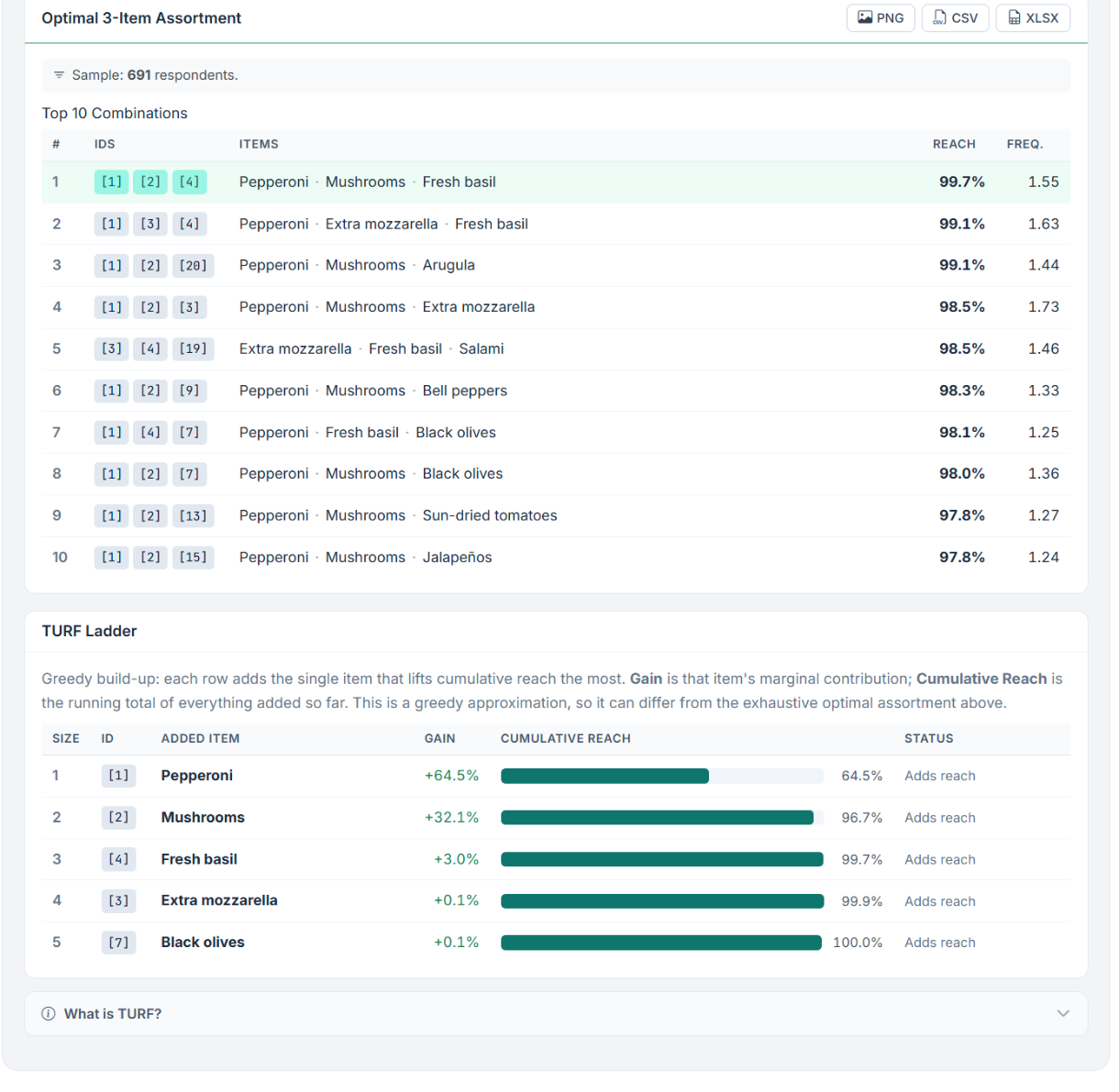
Settings: Assortment Size 3, Reach Definition "top-K" with K = 3, on 312 respondents.
The 6.4-point gap between the naive pick and the TURF pick is the value TURF adds. The numbers are illustrative.
Standard MaxDiff is purely relative: it tells you item A beats item B, but not whether anybody actually wants either. Anchored MaxDiff adds a calibration screen where each respondent answers "Yes" or "No" for every item. Combining the relative HB utilities with those yes/no answers yields an absolute purchase probability per item. This page only appears for anchored runs.
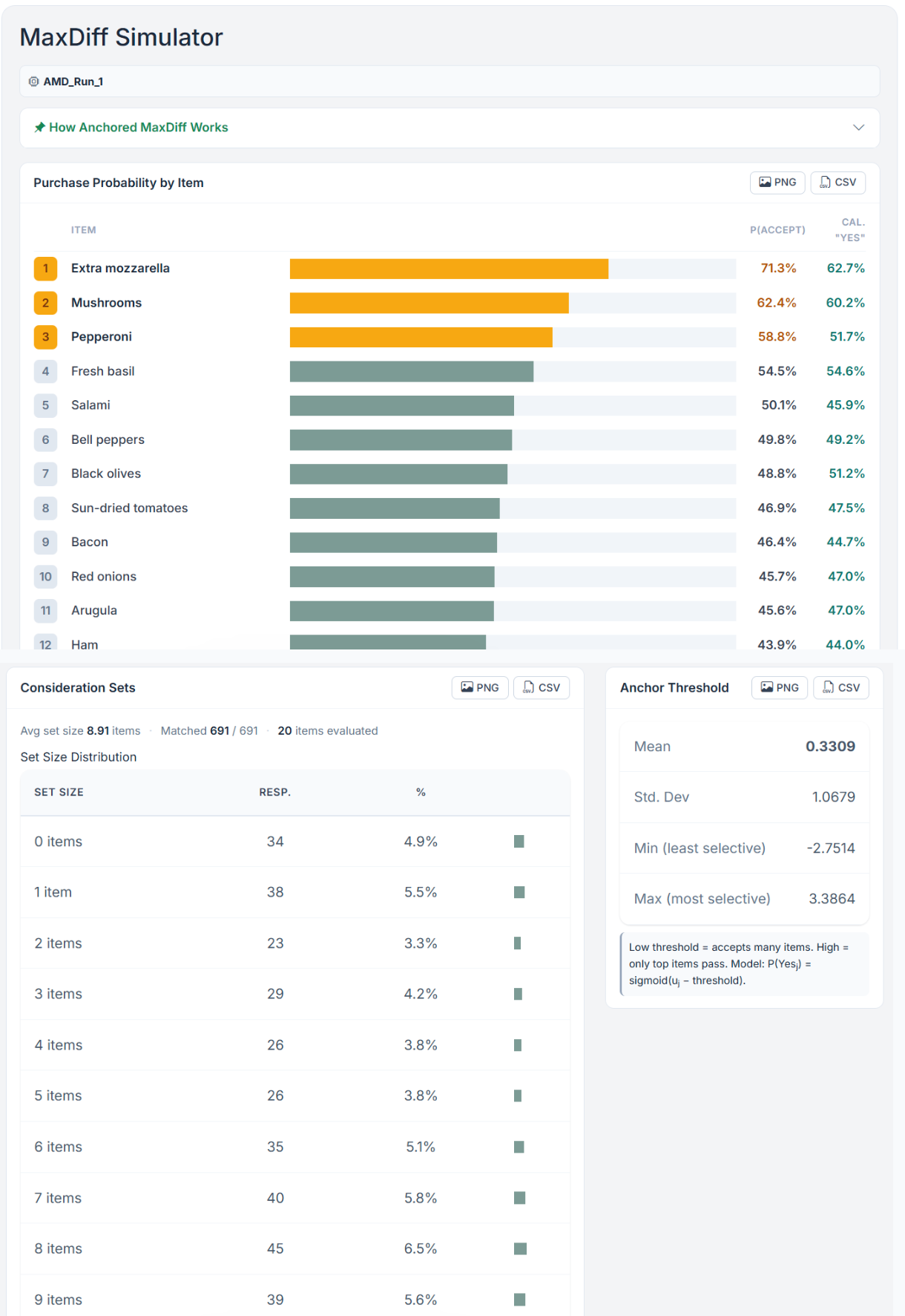
The page opens with a collapsible How Anchored MaxDiff Works panel that summarises the method in two sentences. Below it sit three result cards:
| Card | What it tells you |
|---|---|
| Purchase Probability by Item | Per item, the model's P(Accept) next to the raw calibration "Yes" rate, ranked high to low. P(Accept) is absolute, so it does not sum to 100%. |
| Consideration Sets | The set of items each respondent would realistically consider (P(Accept) above 50%). Shows the average set size, how many respondents matched, and the distribution of set sizes. |
| Anchor Threshold | The per-respondent utility cut-off above which an item is accepted (estimated jointly with the utilities in the HB run, or post hoc by maximum likelihood for TasteNet and older runs). Reports mean, standard deviation, min and max. A low threshold means a respondent accepts many items; a high one means only their very top items pass. |
On anchored runs you also gain two extra reach definitions on the TURF Analysis page: Calibration "Yes" answers (raw), where "reached" means the respondent actually said yes on the calibration screen, and Utility above anchor (model-based), where "reached" means the item's HB-estimated utility exceeds the respondent's anchor threshold. The raw option is the most literal; the model-based option uses the smoothed HB estimate and is robust to single noisy calibration clicks.
Every result on the page can leave it. There are four export channels.
| Button | Where | What you get |
|---|---|---|
| PNG | Each card header | A high-resolution image of that one card, for slides. |
| CSV | Each card header | The card's underlying tables as a spreadsheet-friendly CSV (UTF-8 with BOM). TURF Results includes both the combinations and ladder tables. |
| XLSX | Item Rankings and TURF Results | A multi-sheet workbook (see below). |
| Download PDF | Sidebar, under Report | A formatted PDF report of the whole TURF analysis. |
The Download PDF button appears when results are loaded and your account has export permission for the project (without it the sidebar shows only the Methodology Guide link). If rankings, TURF, or assortment results are not current for the active filters, Choicery prepares them before queuing the report. While rendering, the button becomes Cancel PDF; polling stops after two minutes with a timeout message.
The Item Rankings XLSX exports bundle every metric. Use Summary XLSX for a compact shareable workbook or Full XLSX when respondent-level sheets are required:
The TURF Results XLSX contains:
Definitions, formulas, the optimisation problem, and the literature behind the page.
Let uij be respondent i's utility for item j (probability scale, summing
to 100 over j), and let zij be the same utility zero-centered per respondent.
For a portfolio S, respondent i is reached when any item in S passes the rule.
Selected items contribute jointly. For standard MaxDiff, their exponentiated zero-centered utilities are compared with the other a − 1 alternatives in a MaxDiff set of size a:
Weighted reach has no 100% ceiling to aim for, and its level depends on a. The a − 1 competing alternatives always keep part of the probability, so even the full item set scores below 100%. For a respondent with flat (zero-centered) utilities the full set of n items scores exactly n / (n + a − 1): with 12 items and 5 per set that is 75%. Spread-out utilities push the value above that reference point, and it only approaches 100% for respondents whose preferences are very pronounced. Because a sits in the denominator, the same portfolio scores higher in a study with 3 items per set than in one with 5, so weighted reach levels are not comparable across studies with different set sizes. Compare portfolios within one study, or use a binary rule such as top-K when you need a head count. The TURF results show this reference value for the study at hand whenever Weighted by probability is selected.
For Anchored MaxDiff, the anchor is the comparison alternative. With respondent-specific threshold
ti, use anchored utility zij − ti and denominator 1:
K is capped below the number of items, so an item set can never reach everyone by definition alone.
Finding the best portfolio of size K is a combinatorial optimisation. For n items there are
C(n, K) possible sets. Choicery handles this in two complementary ways.
For the headline result, Choicery enumerates all combinations of the requested size, computes reach and frequency for each, and keeps the best ones. This is exact: it is guaranteed to find the true optimum for that size. To stay responsive it enforces two limits:
| Limit | Value | Why |
|---|---|---|
| Maximum combinations evaluated | 250,000 | Beyond this the search is refused and you are asked to use a smaller size or fewer items. |
| Interactive work budget | 100 million respondent-item evaluations | A search above this is handed to the analysis worker automatically when one is available; the worker runs the same exact search under a larger budget (up to 3 billion evaluations). Without a worker the request is refused with a message. |
| Combinations kept | 10 on the page (API cap 100) | The page asks for the ten best sets; the rest are discarded during the search via a bounded heap. |
Combinations are ranked by reach first, then by frequency as a tie-breaker. The exhaustive search is why very
large assortment sizes on many-item studies can hit the cap: C(40, 8) already exceeds 76 million.
The ladder uses a greedy heuristic instead of exhaustive search. It is the classic algorithm for the maximum-coverage problem:
S = {}                      # empty portfolio
while |S| < ladder_size:
    pick the item j (not in S) that maximises reach(S ∪ {j})
    add j to S
    record reach(S) and the increase
Greedy is fast and intuitive, and it shows the order in which items earn their place. Because maximum coverage is
submodular, the greedy solution is provably within a factor of 1 − 1/e ≈ 63% of the optimum
for that size, and in practice usually much closer. It is therefore a good approximation, but not guaranteed
optimal. When you need the exact best set of a fixed size, read the exhaustive TURF Results table; when you want
to understand the build-up and the diminishing returns, read the ladder.
The Shapley Contribution metric on the Item Rankings page answers a fairness question: "Across all the portfolios an item could belong to, how much reach does it bring on average?" It borrows the Shapley value from cooperative game theory, where players (items) form coalitions (portfolios) and we want each player's fair share of the total value created.
Choicery evaluates contribution with the same portfolio value function used by Weighted TURF. For standard MaxDiff, selected exponentiated utilities enter the portfolio numerator jointly; for Anchored MaxDiff, the anchor is the comparison alternative. The per-item contributions are averaged over respondents and normalised for display.
The exact Shapley value is computed whenever the study is small enough for the full marginal-contribution enumeration. Above that size Choicery switches to a deterministic permutation approximation with a fixed seed, which trades exactness for bounded runtime: the reported contributions then carry a small sampling error, so very close items can swap ranks. When sampling is used, the Shapley card on the Item Rankings page says so and names the number of permutations; the same information is recorded on the Settings sheet of the Item Rankings workbook ("Shapley Calculation" and "Shapley Permutations").
Interpretation: an item with high Shapley contribution pulls its weight in many different portfolios, a hallmark of a versatile, broadly useful item. An item can rank well on Relative Preference yet have a modest Shapley contribution if it mostly duplicates the coverage of more popular items.
Anchored MaxDiff converts the relative HB scale into absolute acceptance probabilities. Choicery estimates, per
respondent, an anchor threshold θi on the utility scale such that an
item is accepted when its utility exceeds the threshold, through a logistic link:
A low threshold means the respondent accepts most items; a high threshold means only their very top items pass. The
Anchor Threshold card reports the mean, standard deviation, minimum, and maximum of θ across
respondents, so you can see how selective your sample is and how much that selectiveness varies.
The model-based P(Accept) usually sits close to the raw calibration "Yes" rate but smooths individual noise, which is why the page shows both side by side. A large, systematic gap between them is a signal to inspect data quality or calibration-screen wording.
Cohen, S. H. (2003). Maximum difference scaling: Improved measures of importance and preference for segmentation. Proceedings of a commercial conjoint software vendor's user conference, 61-74.
Finn, A., & Louviere, J. J. (1992). Determining the appropriate response to evidence of public concern: The case of food safety. Journal of Public Policy & Marketing, 11(2), 12-25.
Louviere, J. J., Flynn, T. N., & Marley, A. A. J. (2015). Best-worst scaling: Theory, methods and applications. Cambridge, England: Cambridge University Press.
Miaoulis, G., Free, V., & Parsons, H. (1990). TURF: A new planning approach for product line extensions. Marketing Research, 2(1), 28-40.
Nemhauser, G. L., Wolsey, L. A., & Fisher, M. L. (1978). An analysis of approximations for maximizing submodular set functions. Mathematical Programming, 14(1), 265-294.
Orme, B. K. (2009). Getting started with conjoint analysis: Strategies for product design and pricing research (2nd ed.). Madison, WI: Research Publishers.
Shapley, L. S. (1953). A value for n-person games. In H. W. Kuhn & A. W. Tucker (Eds.), Contributions to the theory of games (Vol. 2, pp. 307-317). Princeton, NJ: Princeton University Press.
MaxDiff technical methodology paper. Retrieved from vendor documentation.