How to measure and interpret price sensitivity using conjoint-based market simulation, a practical guide for Choicery with methodological background.
Everything you need to measure, interpret, and export price elasticity analyses in Choicery.
Price elasticity measures how much a product’s market share changes when its price changes. It is the single most important metric for pricing decisions: it tells you whether raising or lowering a price will gain or lose customers, and by how much.
An elasticity of −2 means: a 1% price increase leads to a 2% share decrease. The negative sign reflects the law of demand, higher prices typically mean lower demand.
Price elasticity is a property of a product in a market, not of a person or a feature. It depends on which competitors are present and at what prices they are offered. Change the competitive landscape, and the elasticity changes too.
The typical average own-price elasticity across hundreds of consumer-goods studies is about −2.5 (Rao, 2014). However, elasticity varies enormously by category, brand strength, and competitive context, values between −1 and −5 are all common.
Before running Price Elasticity in Choicery, make sure you have the following:
A completed analysis run with individual-level utilities. Price elasticity is computed via market simulation, which requires individual-level part-worth utilities. Choicery accepts a completed Preference Analysis (HB) run or a completed AI-Driven Profile Analysis run. Pick the run you want in the Run dropdown at the top of the Market Simulation page. Without a completed run, the Price Elasticity tab is disabled.
A price attribute declared under Price Setup. Your conjoint design must include a price attribute. A linear (continuous) price attribute is preferred for smooth elasticity curves, but categorical price levels also work. Open Price Setup in the top bar of the Market Simulation page and set the global price attribute. The Price Elasticity tab has no price-attribute dropdown of its own: it shows a read-only badge reading “Price Attribute: … · from Price Setup”.
Products defined in the Products panel. With no products, the Price Elasticity controls are greyed out and the tab shows “Add at least one product in the Products panel to use Price Elasticity.” One product plus the None alternative is technically enough for an own-price curve, but elasticity is only meaningful against a realistic competitive set. Cross-price elasticity needs at least two products.
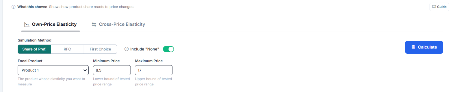
Open Market Simulation and switch to the Price Elasticity tab. The tab bar on the right-hand panel reads Choice Share, WTP, Reservation Price, Price Elasticity, Sensitivity, Persona. Inside the Price Elasticity tab, two sub-tabs select the analysis type: Own-Price Elasticity and Cross-Price Elasticity. Each sub-tab keeps its own results, so you can switch back and forth without recalculating.
The Focal Product is the product whose price will be varied. All other products remain at their defined prices, and every product in the Products panel competes. Minimum and Maximum Price are pre-filled with the observed price range of the selected price attribute whenever Choicery can infer it. The elasticity is calculated for exactly the values in these fields: values you enter stay when you switch tabs or apply Price Setup, and the fields are refilled only when they are empty or the price attribute changes. The demand curve’s x-axis runs from the minimum to the maximum price. If you enter values outside the observed range, Choicery computes the run anyway and adds the note “Prices outside the estimated range X to Y were extrapolated. Utilities beyond the design are an assumption of the model, not something the data shows.” to the warnings at the bottom of the tab.
If any product has no price value set, the calculation stops with “Price value missing for product(s): ...”, listing the product numbers. Minimum and Maximum Price replace the price of the focal product only; every other product needs its own price.
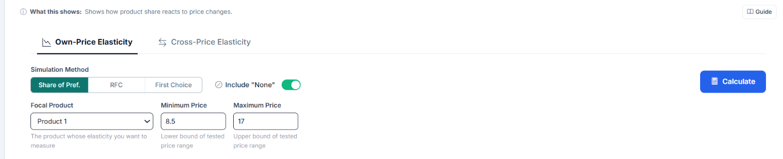
Click Calculate to run the simulation. Choicery then performs three passes with the same settings:
The log-log pass requires strictly positive prices. If the minimum price is zero (or negative, which is only possible with Allow negative prices on), the Log-Log Summary Fit (Average Elasticity) card shows a dash with the label N/A and the R² card shows a dash, while arc elasticity and the demand curve are still shown.
The results block is headed Elasticity Results. Next to the heading, a small chip reports which respondents were used: “n=… (… unusual price responses excluded)” by default, or “All respondents n=…” when Include unusual price responses in price analyses is on in Analysis Settings. On the right sits the Excel download button.
Four metric cards are displayed:
| Metric | Description |
|---|---|
| Arc Elasticity | A single number summarizing the two-point (midpoint method) elasticity between the minimum and maximum price. Symmetric: the same result whether you go from low-to-high or high-to-low. |
| Log-Log Summary Fit (Average Elasticity) | The constant elasticity estimated by regressing ln(share) on ln(price) across the seven simulated price points. It is a summary fit over the whole tested range, not the elasticity at any single price: a logit share curve is not iso-elastic, so check R² before quoting it as one number. More stable than arc elasticity because it uses more than two points. Own-price only. |
| R² (Log-Log) | The coefficient of determination of the log-log regression. Values close to 1.0 indicate the constant-elasticity model fits the demand curve well. Low R² suggests the elasticity changes substantially across the price range. |
| Price Change (midpoint) | The percentage price change between minimum and maximum price, computed on the midpoint basis used for arc elasticity. The line underneath reads “Share Change (midpoint)” and gives the matching share change. |
Below the cards, an interpretation banner spells the result out in words, for example “Elastic demand (|E| > 1): A 1% price increase leads to a …% decrease in simulated preference share.” Inelastic results read “Inelastic demand (|E| < 1): ...”, a flat curve reads “Flat simulated demand: ...”, and a positive value reads “Positive own-price elasticity: Share rises as price increases. Review the price coding and demand curve. The Revenue Rule is not applied to this result.”

For conventional downward-sloping own-price demand (E < 0), the magnitude is read from the absolute value |E|. The label under each card is Elastic (|E| > 1), Inelastic (|E| < 1), Unit Elastic (|E| exactly 1) or Positive / Unusual (E > 0). The Interpretation row of the Excel Summary sheet is finer grained: it is written from a four-band classification (“highly price-sensitive”, “price-sensitive”, “relatively price-insensitive”, “highly price-insensitive”) with these cut-offs:
| |E| Range | Classification | Meaning |
|---|---|---|
| |E| > 1.5 | Highly elastic | Very price-sensitive. Small price changes cause large share swings. |
| 1 < |E| ≤ 1.5 | Elastic | Price-sensitive. Share responds more than proportionally to price changes. |
| 0.5 < |E| ≤ 1 | Inelastic | Price-insensitive. Share responds less than proportionally to price changes. |
| |E| ≤ 0.5 | Highly inelastic | Barely price-sensitive. Large price moves shift share only marginally. |
If own-price elasticity is positive, simulated share rises as price increases. Choicery marks the result as Positive / Unusual. Review the price coding and demand curve before interpreting it, and do not apply the usual Revenue Rule.
If |E| > 1 (elastic): raising price decreases total revenue, the volume you lose outweighs the extra revenue per unit.
If |E| < 1 (inelastic): raising price increases total revenue, you lose some volume, but each unit earns more, and the net effect is positive.
This rule applies only when own-price elasticity is negative and demand slopes downward.
Below the summary metrics sits the Demand Curve block, subtitled “Simulated preference share at different price points”. It is a line chart showing how simulated preference share (Y-axis) varies as the focal product’s price (X-axis) changes. This visual is the most intuitive way to understand price sensitivity: a steep, rapidly dropping curve means the product is highly price-elastic; a gently sloping curve means it is relatively price-insensitive.
Two buttons in the header of that block export the chart: CSV and PNG. Both work for own-price and for cross-price curves.
If filters are applied through the Filters button in the left panel, the chart draws one curve per selected group in addition to the full sample, and a row of filter pills above the chart lets you show and hide individual curves. The pills only appear when there are at least two curves.
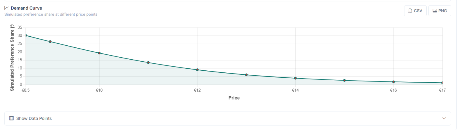
Under the chart, the Show Data Points button expands a table with the raw simulation data. It has three columns: Price, Simulated Preference Share (%) and Local Arc Elasticity. The last column is the midpoint-formula elasticity between neighbouring simulated price points (central difference inside the curve, one-sided at the two ends), so it is a local arc value, not a derivative. This is useful for checking where along the range the elasticity changes.
If price was estimated as a categorical attribute, a note at the bottom of the tab lists the observed price levels and states that elasticity is interpolated between them, and that values outside that range are treated as extrapolation.
In cross-price analysis, the focal product’s price stays fixed while the competitor product’s price is varied. Competitor minimum and maximum price are pre-filled from the observed price range when available and keep the values you enter; values outside that range are treated as extrapolation. The question being asked is: “When Product B gets more expensive, how much share does Product A gain?”
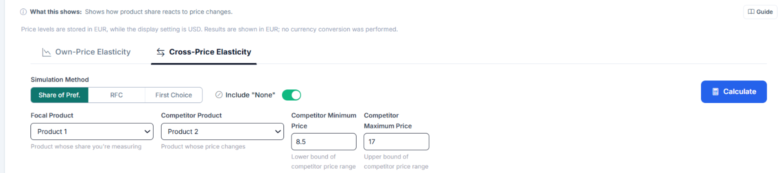
Cross-price elasticity is reported as a single arc value in the Arc Elasticity card, plus a Cross-Price Demand Curve showing how the focal product’s share changes as the competitor’s price moves. The curve subtitle also states the focal product’s fixed price.
No log-log regression is run in cross-price mode, so the Log-Log Summary Fit (Average Elasticity) card shows a dash with the label “N/A” underneath, and the R² card shows a dash as well. The Excel button is hidden in this sub-tab; the curve CSV and PNG buttons remain available.
| Cross-Elasticity Value | Classification | Meaning |
|---|---|---|
| > 0.5 | Strong substitute | The focal product gains substantial share when the competitor raises prices. These products compete head-to-head. |
| 0.1 to 0.5 | Substitute | Some competitive relationship exists. Price changes in one affect the other moderately. |
| −0.1 to 0.1 | Independent | Negligible competitive interaction. These products serve different customer needs. |
| −0.5 to −0.1 | Complement | The focal product loses share when the competitor raises prices. Rare in conjoint but theoretically possible (bundled goods, ecosystem effects). |
| < −0.5 | Strong complement | A large negative reading. In a conjoint scenario this usually points to a configuration problem rather than a genuine complement relationship. Check the product setup. |
The card label under the value is coarser: it reads Substitute above 0.1, Complement below −0.1, and Independent in between.
Run cross-price elasticity for your focal product against each competitor in turn. The competitor with the highest cross-price elasticity is your closest substitute, the one that gains the most when you raise prices, and the one you gain the most from when they raise theirs.
The demand curve is the most intuitive visualization of price sensitivity. Here is how to read it:
In the Cross-Price Elasticity sub-tab the same chart is titled Cross-Price Demand Curve and the X-axis carries the competitor’s price, while the Y-axis still shows the focal product’s share. There, an upward slope is the expected pattern for substitutes.
| Curve Shape | Elasticity | Interpretation |
|---|---|---|
| Steep drop-off | Highly elastic | Share crashes with small price increases. The product competes primarily on price. |
| Gentle slope | Inelastic | Share changes little with price. The product has strong non-price differentiation (brand, features). |
| S-shaped / concave | Varies along curve | The product is inelastic in a “sweet spot” and becomes elastic at extreme prices. Check the log-log R², if low, elasticity is not constant. |
When filters are active (the Filters button in the left panel), Choicery overlays a separate demand curve per filtered group on the same chart, alongside the full sample, and reports a per-group elasticity block above the chart. This is useful for pricing strategy: you may discover that one group is highly price-elastic while another is inelastic, suggesting that a differentiated pricing strategy or a product line with premium and value tiers could increase total revenue.
The Excel button in the Elasticity Results header exports the workbook. It is available for own-price elasticity only; the button is hidden in the Cross-Price Elasticity sub-tab. The file is named price_elasticity_<timestamp>.xlsx and contains three sheets:
point_elasticity, kept under that name for compatibility).The CSV and PNG buttons in the Demand Curve header work in both sub-tabs. The CSV is written as demand_curve.csv (own-price) or cross_price_demand_curve.csv (cross-price), with the columns Sample, Price (or Competitor Price), Share (%) and Local Arc Elasticity. When filters are active, each filtered group is written as its own Sample block.
The exports are useful for creating custom visualizations, incorporating elasticity data into pricing models, or sharing results with stakeholders who do not have access to Choicery.

Conjoint-based elasticities are directionally correct and excellent for relative comparisons (Product A is twice as elastic as Product B). However, their absolute magnitudes should be treated as lower bounds. In-market elasticities are typically 1.5 to 2× larger because real consumers face budget constraints that survey respondents do not (Orme, 2020).
The mathematical foundations behind price elasticity measurement in conjoint-based market simulation.
Arc elasticity uses the midpoint method to compute elasticity between two price-share observations. The key advantage over simple percentage change is symmetry: the elasticity from point A to point B is identical to the elasticity from B to A.
Where:
Suppose a coffee brand has the following simulated market shares:
Interpretation: The elasticity is −1.08, meaning the product is slightly elastic. A 1% price increase leads to roughly a 1.08% share decrease. Since |E| > 1, a price increase would decrease total revenue (adapted from Orme, 2020).
When more than two price points are available (Choicery simulates seven evenly spaced points across the tested range for this purpose), a more robust approach is to fit a constant-elasticity model via log-log regression:
In this model:
Arc elasticity uses only the two extreme points and ignores everything in between. Log-log regression uses all seven simulated price points, producing a more stable estimate. It also has a natural interpretation: the coefficient is a direct elasticity reading. The trade-off is that it assumes constant elasticity, always check R² to verify this assumption.
If R² is low (e.g., below 0.90), the demand curve has a shape that the constant-elasticity model cannot capture well, for example, an S-curve where elasticity is low in the middle of the price range and high at the extremes. In such cases, report the full demand curve rather than a single elasticity number, and consider narrowing the price range to a region where the constant-elasticity fit improves.
Cross-price elasticity measures competitive interaction between products:
In standard MNL-based simulation (including Share of Preference), cross-price elasticities follow the Independence of Irrelevant Alternatives (IIA) property: when one product loses share, it is distributed proportionally to all remaining products based on their current shares. This means MNL cross-elasticities may not capture asymmetric substitution patterns. Individual-level HB utilities partially mitigate this, but the limitation remains (Train, 2009).
For a market with N products, the full cross-elasticity matrix is an N×N table where entry (j, k) gives Ejk. The diagonal entries are own-price elasticities (negative). Off-diagonal entries are cross-price elasticities (typically positive). Products in the same row that have high cross-elasticities are close substitutes for the focal product.
The Revenue Rule is arguably the most practically important consequence of price elasticity. It connects elasticity directly to the profit impact of pricing decisions.
The standard rule assumes conventional downward-sloping own-price demand (E < 0). If the estimated elasticity is positive, review the price coding and demand curve instead. Choicery does not apply the Revenue Rule to that result.
When you raise a price, two opposing forces act on revenue:
Which force wins depends entirely on elasticity:
| Condition | Price Increase Effect | Price Decrease Effect | Why |
|---|---|---|---|
| |E| > 1 (elastic) | Revenue decreases | Revenue increases | Volume loss outweighs per-unit gain. Customers are sensitive (many leave). |
| |E| < 1 (inelastic) | Revenue increases | Revenue decreases | Per-unit gain outweighs volume loss. Customers are sticky (few leave). |
| |E| = 1 (unit elastic) | Revenue unchanged | Revenue unchanged | The two effects exactly cancel. This is the revenue-maximizing price. |
Consider two products in a market of 10,000 potential customers:
Key insight: The same 10% price increase produced opposite revenue outcomes. For the inelastic Product A, raising price was profitable. For the elastic Product B, it was destructive. This is why measuring elasticity before making pricing decisions is essential.
In theory, the revenue-maximizing price is where |E| = 1 (unit elastic). In practice, firms optimize profit (revenue minus cost), not just revenue. The profit-maximizing price depends on the margin: higher-margin products can tolerate more elastic demand. The general rule is that the optimal markup over marginal cost equals 1/|E|, this is the Lerner Index from microeconomic theory.
Orme, B. K. (2020). Getting started with conjoint analysis (4th ed.). Manhattan Beach, CA: Research Publishers LLC.
Orme, B. K., & Chrzan, K. (2017). Becoming an expert in conjoint analysis. Orem, UT: Commercial conjoint software publisher
Rao, V. R. (2014). Applied conjoint analysis. Berlin: Springer.
Train, K. E. (2009). Discrete choice methods with simulation (2nd ed.). Cambridge: Cambridge University Press.