How to discover and profile consumer segments with finite mixture models. Every setting of the form, how to read the results, and the method behind it, with the pizza oven CBC of the Pizza (Example) study as worked example.
Everything you need to run, interpret, and export Latent Class analyses in Choicery.
1. What Is Latent Class Analysis?
Latent Class (LC) analysis discovers hidden consumer segments in your conjoint data. Instead of assuming everyone has the same preferences (aggregate logit model) or that everyone is unique (HB individual-level model), LC finds a middle ground: a small number of discrete segments, each with its own distinct preference profile.
Think of it as running a cluster analysis and a logit estimation at the same time. The model simultaneously identifies the segments and estimates the preference weights (part-worth utilities) that characterize each segment (Orme & Chrzan, 2017).
The core idea
Your respondents don’t all think alike. Some are price-sensitive, some are brand-loyal, and some care primarily about features. LC discovers these groups automatically from observed choice patterns, without you having to specify them in advance.
Key Output
Segment-specific part-worth utilities, a full utility profile for every attribute level within each discovered segment.
Segment sizes, how large each segment is (as a proportion of the total sample).
Individual class membership probabilities, for every respondent, the probability of belonging to each segment.
Why “Latent”?
The segments are latent (hidden) because you cannot observe them directly. A respondent does not carry a label saying “I am in the price-sensitive segment.” Instead, their membership is inferred from the pattern of choices they made. This makes LC a post hoc, behavior-based segmentation approach, segments emerge from choice data, not from demographics or pre-defined groups.
LC vs. traditional segmentation
Traditional segmentation (e.g., “Millennials vs. Boomers”) is based on observable variables chosen by the researcher. LC segmentation is based on revealed preferences, the model finds the grouping that best explains the heterogeneity in choice behavior. You can then profile the segments with demographics after the fact.
2. Prerequisites
Before running Latent Class in Choicery, make sure you have the following:
1
A completed conjoint task with collected responses. LC runs independently from HB estimation, it works directly on raw choice data. However, the conjoint task and its experimental design must already exist in your project.
2
At least ~100 respondents. LC estimates multiple sets of parameters simultaneously (one full set per class), so it requires more data than a simple aggregate model. With fewer than 100 respondents, class solutions may be unstable. More respondents (200+) lead to more reliable segment identification.
3
Navigate to Conjoint Analysis → Latent Class tab. From your project, go to Analysis → Conjoint Analysis. At the top of the page you will see four tabs: Preference Analysis (HB), AI-Driven Profile Analysis, Latent Class, and Interaction Effects. Click Latent Class.
4
Know the three workflow steps. Below the tab row, Latent Class runs through a stepper with three steps: 1 Estimation, 2 Results, and 3 Export. A funnel button to the left of the stepper opens the Participant Filter, and a Methodology Guide button on the right opens this document.
Sample size rule of thumb
A rough guideline: you need at least 50 to 100 respondents per class for stable estimates. If you suspect 4 classes, aim for 200 to 400 respondents. With small samples, you may find that the optimal number of classes is artificially constrained, the data simply cannot support fine-grained segmentation.
3. Running LC in Choicery
3.1 Creating a Run
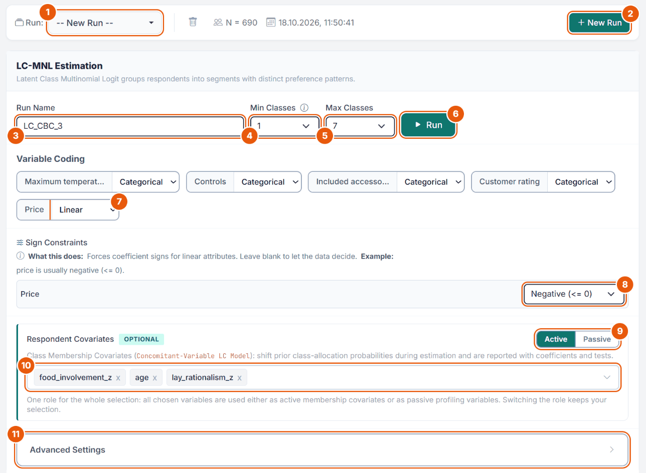
The estimation form sits in a card titled LC-MNL Estimation. Figure 1 shows it for the pizza oven CBC (cbc_pizza_oven, 690 respondents) with the settings used throughout this guide: price coded linear with a negative sign, and three respondent characteristics as active membership covariates.
Figure 1. The Latent Class form of the Pizza task cbc_pizza_oven.
No.
Control
What it does
1
Run
Lists the saved runs of this task. Pick one to view its settings and results; the bin icon next to it deletes the selected run. The bar also shows N and the start time of the run.
2
New Run
A completed run is shown read-only. New Run unlocks the form for the next run and keeps the coding, sign constraints, covariates and Advanced Settings of the run you were looking at.
3
Run Name
Suggested per task type (LC_CBC_1, LC_MD_1 for MaxDiff, LC_AMD_1 for Anchored MaxDiff, LC_DRCBC_1 ...). Up to 50 characters.
4
Min Classes
Smallest multi-class model to estimate (1 to 10, default 1).
5
Max Classes
Largest model to estimate (1 to 10, default 5). The Pizza example uses 7.
6
Run
Starts the estimation (section 3.5).
7
Variable Coding
Categorical or Linear per attribute (section 3.2). Linear opens fields for the numeric value of every level; Choicery fills them from the level labels (69, 139, 209, 279 for the Pizza prices).
8
Sign Constraints
Appears once an attribute is Linear: no constraint, Positive (>= 0) or Negative (<= 0).
9
Active / Passive
Decides what the selected covariates are used for (section 3.3).
10
Covariate picker
Opens the variable list with search and type tags. The list loads when you open it the first time.
11
Advanced Settings
EM settings, validation and weighting (section 3.4).
Choicery estimates all models from the minimum to the maximum number of classes. For example, with Min = 2 and Max = 5 it estimates the 2-, 3-, 4-, and 5-class models. It then selects the model with the lowest BIC automatically.
The 1-class aggregate model (pooled MNL) is always estimated as a reference, in addition to the range you set. With Min = 2 and Max = 5 the estimated set is therefore {1, 2, 3, 4, 5}. This gives every fit statistic a common baseline, and it is why a 1-class Latent Class fit is identical to an aggregate MNL.
If you set Min above Max, the form shows “Minimum classes must be less than or equal to maximum classes.” and disables the Run button.
Choicery keeps at most 10 Latent Class runs per conjoint task; when the limit is reached the message “Maximum of 10 runs per task reached. Please delete an existing run before starting a new one.” appears. Failed and cancelled runs keep their names reserved until you delete them.
3.2 Variable Coding and Sign Constraints
For each attribute in your conjoint design, you can choose how it is coded in the LC model:
Coding
When to Use
What It Does
Categorical (default)
Most attributes (brand, color, features)
Effects-coded, one utility per level, sum-to-zero constraint. This is the standard approach.
A single linear coefficient per attribute. Every level needs a numeric value; Choicery fills them from the level labels where it can, so check them before you run. Reduces the number of parameters, useful when linearity is a reasonable assumption.
When to use linear coding
Linear coding is appropriate for price and other quantitative attributes where you expect a monotonic relationship (higher price → lower utility). It uses one parameter instead of L − 1, which can improve model stability with many levels. However, if the relationship is non-linear (e.g., a U-shaped effect), categorical coding is safer.
Sign Constraints
A Sign Constraints section appears as soon as at least one attribute is set to Linear. For each linear attribute you can choose No sign constraint (the default), Positive (>= 0), or Negative (<= 0). The help text in the app puts it plainly: “Forces coefficient signs for linear attributes. Leave blank to let the data decide.” Price is the usual candidate for a negative constraint.
Task-specific checkboxes
Include None Option appears for DR-CBC and for BW-CBC with a none option in the design. It folds the task’s follow-up no-choice signal into the model. Disable it to estimate from the product-choice stage only.
Estimate Display Position Effects appears for CBC Shop only. It adds control terms derived from the rendered product order, which helps separate position effects from product-attribute utilities.
For CBC and CBC Shop designs that contain a none option there is no checkbox: the none alternative is always part of the model and reported as a separate ASC (NoneOpt or ASC_none) outside the attribute tables and importances.
3.3 Respondent Covariates: Active or Passive
Choicery offers one optional Respondent Covariates picker with a global Active / Passive switch (markers 9 and 10 in Figure 1). There is a single selection of variables, and the switch decides what the whole selection is used for. The two roles are never mixed within a run, and switching the role keeps your selection.
Active: Class Membership Covariates (Concomitant-Variable LC Model). They shift the prior class-allocation probabilities during estimation and are reported with coefficients and tests.
Passive: Class Profiling Variables. They describe the fitted classes without changing class allocation or the likelihood.
For the Pizza example the active covariates are food_involvement_z (how much someone cares about food), lay_rationalism_z (how strongly someone decides by “hard” facts such as price) and age: three characteristics that plausibly change what someone wants from a pizza oven. Use scale scores where you have them; single grid items or open answers are poor membership covariates.
With Active covariates the model becomes a Concomitant LC-MNL: class membership probabilities become respondent-specific functions of the selected covariates (see Section 13 for the mathematical details). With Passive covariates the estimation is a standard LC-MNL and the variables are used only to describe the resulting classes.
Numeric variables (age, income) are mean-imputed, then z-standardized with the population standard deviation before entering the model.
Categorical variables (gender, education) are mode-imputed and dummy-coded; the alphabetically first level is the reference level and is dropped.
Variables that are constant after imputation, or that produce no usable dummy, are dropped and listed under Dropped in the Class Membership Model card. Imputation counts are recorded with the run and shown in the feature notes.
When to use active membership covariates
Use them when you have a strong prior belief that demographics or attitudes are related to segment membership. Start with 3 to 5 well-chosen variables. Too many covariates relative to sample size can cause estimation instability.
3.4 Advanced Settings
A collapsible Advanced Settings panel at the bottom of the estimation card provides additional controls.
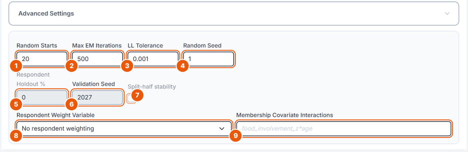
Figure 2. Advanced Settings of the Pizza run LC_CBC_3. Holdout and split-half are greyed out because active covariates are selected.
No.
Field
What it does
1
Random Starts
Random EM starts per class count (1 to 100, default 5); the best-fitting start is kept. 5 is fine for exploring, use 10 to 20 for final results. The Pizza run uses 20.
2
Max EM Iterations
Upper bound on EM iterations per start (10 to 5000, default 100). Raise it if a solution is reported as provisional. The Pizza run uses 500.
3
LL Tolerance
Convergence threshold (0.00000001 to 0.01, default 0.001): the EM stops once the log-likelihood improves by less than this value.
4
Random Seed
Seeds the random starts (default 1), so the same settings give the same result. Change it to check that a solution is stable.
5
Respondent Holdout %
Percent of respondents (0 to 49) held out of estimation to check out-of-sample fit. The Results step then reports the holdout log-likelihood and Pct Certainty from a separate training fit.
6
Validation Seed
Seeds only the holdout and split-half draws (default 2027). Greyed out until a holdout percentage or split-half is requested.
7
Split-half stability
Refits the selected specification on two random respondent halves and compares the matched classes.
8
Respondent Weight Variable
Optional positive survey or frequency weight. Values must be complete and greater than zero; weights are normalized to mean 1. Weighted runs use a pseudolikelihood, information criteria become heuristic, and non-robust Wald inference is withheld.
9
Membership Covariate Interactions
Optional first-order interactions written as Variable A*Variable B and separated by commas; both main effects must be selected as Active covariates. The field stays disabled until two active covariates are selected and then suggests the first pair, here food_involvement_z*age.
Active covariates disable the validation options
Selecting Active covariates greys out Split-half stability and Respondent Holdout %, and resets them. A concomitant model would need a separately fitted membership model per half, and a full-sample membership model would leak holdout information. Switch the role to Passive if you need those checks.
3.5 Running the Estimation
1
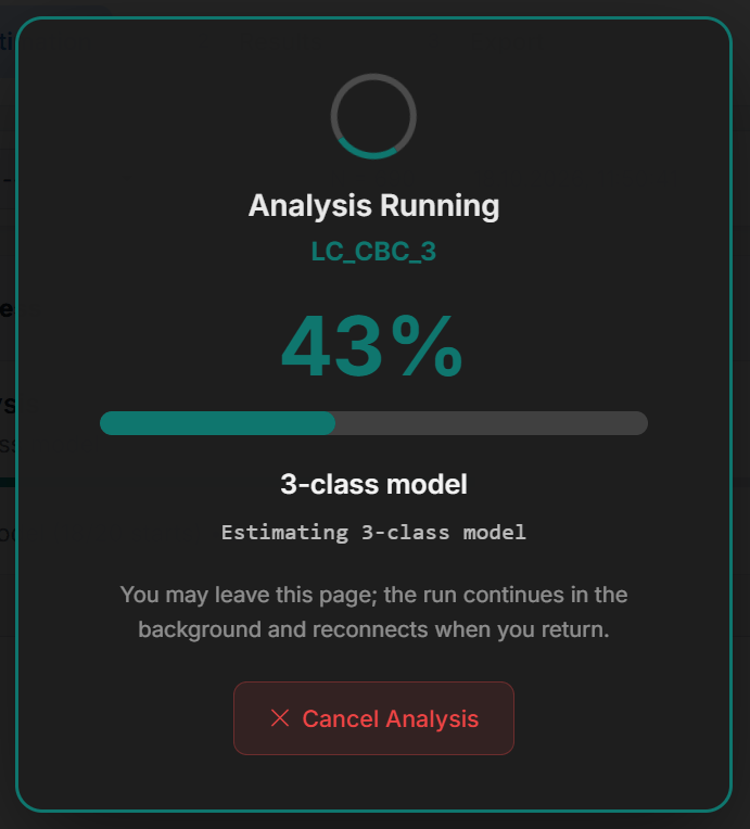
Click Run. A full-screen panel Analysis Running shows the run name, the percentage and the current step, for example “Estimating 3-class model” (Figure 3). Underneath, the LC Estimation Progress card adds the start counter, for example “Estimating 4-class model (2/20 starts)”. You may leave the page; the run continues in the background and the page reconnects when you return.
Figure 3. The Pizza run LC_CBC_3 while it estimates the 3-class model.
2
Cancel Analysis stops the run at any time. Cancelling aborts the whole run: it is marked as cancelled and no partial results are stored.
3
When the run is complete, Choicery switches to the Results step by itself and shows the model with the lowest BIC.
Estimation time
Estimation time grows with the sample, the number of parameters, the class range and the number of starts. The Pizza run LC_CBC_3 (690 respondents, 1 to 7 classes, 20 starts each, three active covariates) took about 7 minutes; the same task with 1 to 5 classes and 10 starts took about 2 minutes. Concomitant runs add a final membership-inference step after the class solutions.
4. Interpreting Results
4.1 Meta Bar and the Ready-to-Report Gate
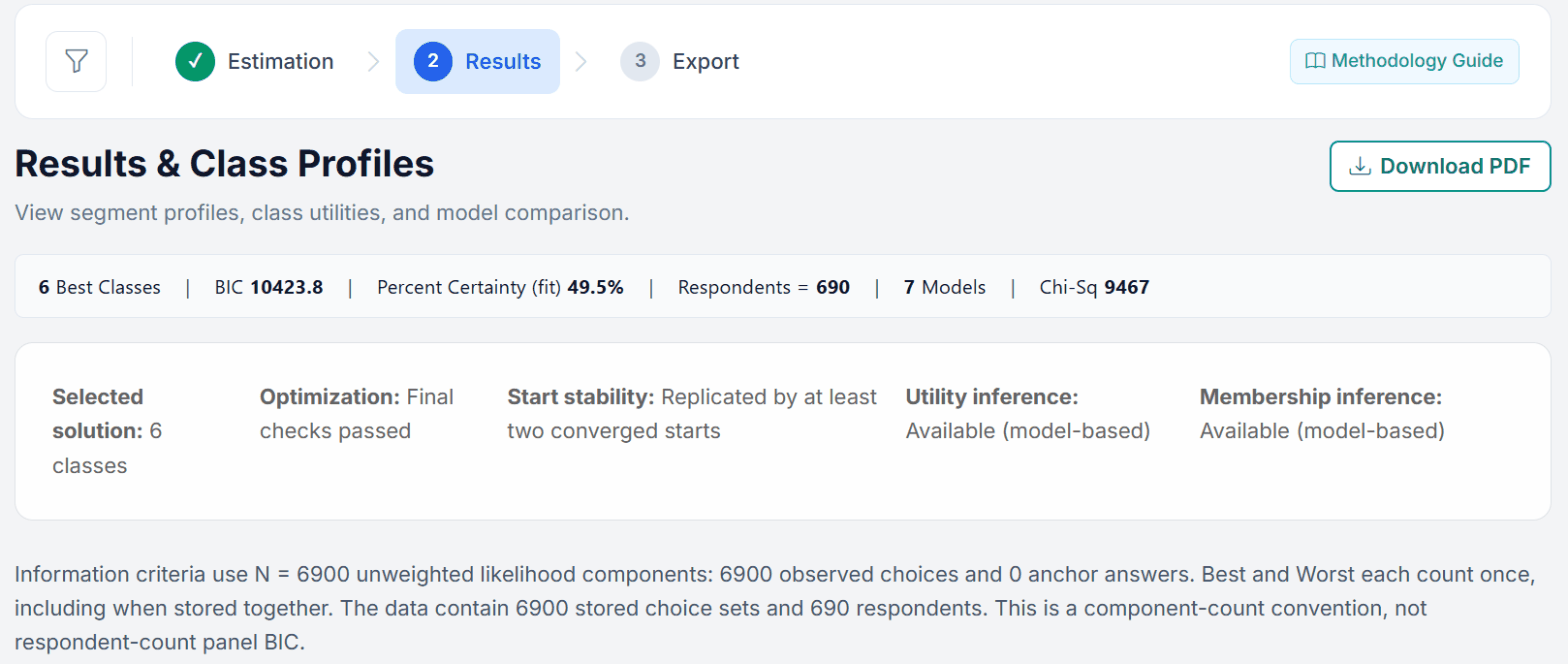
The Results step opens with a one-line meta bar summarizing the run: Best Classes, BIC, Percent Certainty (fit), Respondents, the number of estimated Models, and Chi-Sq. Below it sit the Solution diagnostics box and, where needed, yellow warnings (Figure 4; the Pizza run needs none).
Figure 4. Top of the Results step for the Pizza run LC_CBC_3. The 6-class model has the lowest BIC and passes every check.
Pct Cert is 100 × (1 − model log-likelihood / null log-likelihood). It is a descriptive fit improvement, not a classification certainty.
Chi-Sq is 2 × (model log-likelihood − null log-likelihood). It is descriptive for finite-mixture class solutions; no standard chi-square p-value is implied.
The Solution diagnostics box is the reliability gate. It always describes the solution selected in the Class Solution card (section 4.3), so it changes when you switch solutions:
Solution diagnostics
Directly below the meta bar, a Solution diagnostics box summarizes the currently selected class solution in five rows: Selected solution, Optimization (Final checks passed, or Provisional or final checks unavailable), Start stability (Replicated by at least two converged starts, Near-best starts disagree, Insufficient independently converged replications, or Final reference solution is provisional), Utility inference and Membership inference (Available, Withheld, or Not recorded). The final checks evaluate the observed-data score norm at the reported parameters, normalized per model observation, against a limit of 1e-3 per observation, and require no likelihood decrease and no rejected optimizer update (Section 10.2). Finished EM starts and final diagnostics are separate checks: a model can have all starts finished and still be provisional.
Underneath, one or more yellow warnings can appear: “The selected solution is provisional. Continue optimization before final reporting.”, “Possible separation or a degenerate class: review coefficient magnitudes and class sizes.”, a Small-class sample warning naming the smallest expected class against the recommended minimum of 30 respondents, and “Start stability is not established.” The recommended reaction to a provisional solution is a new run with a higher Max EM Iterations (for example 500 or more) and a stricter LL Tolerance (for example 0.0001); if the warning persists, report the lowest-BIC model among the rows marked Yes under Ready to Report. The raw values (Provisional, Stationary Diagnostics, Separation Suspected) are in the Model Comparison CSV.
Pizza example: what the diagnostics say
For the BIC-selected 6-class solution the box reads Optimization: Final checks passed and Start stability: Replicated by at least two converged starts, and no warning appears: the solution can be reported. Switching to the 5-class solution shows a different picture: Start stability: Insufficient independently converged replications together with the warning “Start stability is not established.” All 20 starts converged there too, but only one of them reached the best log-likelihood; the next best ended about 3 log-likelihood points lower. A second run with another Random Seed would show whether that solution is reproducible.
Other banners you may see, depending on the run:
Possible separation or degenerate class, when coefficient magnitude or minimum class-share diagnostics crossed the guardrail.
Requested membership model was not estimated, when covariate alignment or encoding failed and the run fell back to standard LC.
Respondent-weighted pseudolikelihood, when a weight variable was used.
Respondent holdout and Split-half stability, reporting the validation results or the reason they could not be computed.
Anchored MaxDiff calibration included and Relative Worst scale notices for the corresponding task types.
4.2 Model Comparison
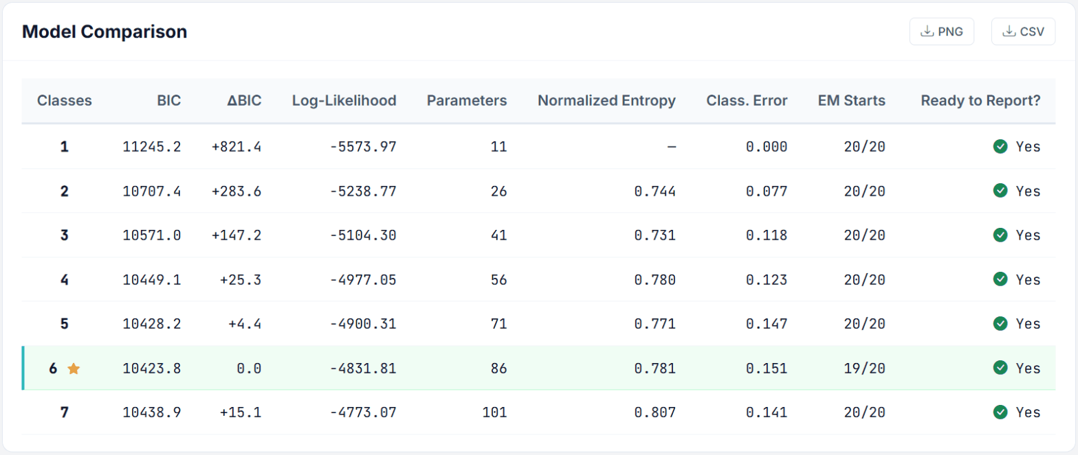
The Model Comparison card summarizes all estimated models side by side. The row of the BIC-selected model is highlighted and carries a star.
Figure 5. Model Comparison of the Pizza run LC_CBC_3.
In the Pizza run the BIC falls up to 6 classes and rises again at 7, so the minimum lies inside the range. A first run with Max Classes 5 had its lowest BIC at the upper end of the range, which is the signal to widen it. The 6-class model is selected and marked Yes under Ready to Report?; the rest of this chapter shows it. The 5-class model is only 4.4 BIC points worse. Such a small gap means both solutions describe the data almost equally well; compare their segments before deciding, and prefer the smaller one if the extra class adds nothing you can act on. When a row says No, its tooltip names the reason, for example “The final stability or identification checks did not pass.”
Columns explained:
BIC: Bayesian Information Criterion. Lower BIC = better model. Penalizes complexity more heavily than AIC, tending to favor more parsimonious solutions.
ΔBIC: BIC difference to the best model. The best model shows 0.0.
Log-Likelihood: The log-likelihood at convergence. Higher (less negative) is better, but it always improves with more classes, which is why information criteria are used for selection.
Parameters: Number of free parameters. More classes = more parameters = more complex model.
Normalized Entropy: Entropy R², a 0-to-1 measure of how cleanly respondents separate into classes. Higher is better separation. It is a description of the solution, not a selection criterion.
Class. Error: Posterior expected modal-assignment error, that is 1 minus the weighted mean of each respondent’s largest posterior class probability. It is not an observed misclassification rate.
EM Starts: Random starts that met the EM stopping rule, out of the total number of starts requested.
Ready to Report?: Yes only when three things hold at once: the model met the EM stopping rule, it passed the final stability and identification checks described in Section 4.1, and its smallest class has an expected size of at least 30 respondents (prior share times respondent N). A No caused by class size is explained in the cell tooltip, and the Class Solution card shows a Small-class sample warning for the affected solution.
The card’s CSV button exports a wider table than the one on screen, but not an exact superset of it. The CSV drops ΔBIC, and it replaces Class. Error, EM Starts and Ready to Report? with the underlying raw fields. Its columns are Classes, Log-Likelihood, Pct Cert, Parameters, BIC, CAIC, AIC, AIC3, ABIC, Entropy, Normalized Entropy, Estimated Assignment Error, Chi-Square, Relative Chi-Square, Converged, Converged Starts, Total Starts, Provisional, Stationary Diagnostics and Separation Suspected. A PNG button downloads the card as an image. Several other result cards carry a PNG or CSV button of their own.
Choosing the right number of classes
BIC is the primary criterion, but also consider: (1) is the model marked Ready to Report? (2) interpretability, can you tell a meaningful story about each segment? (3) segment sizes, are all segments large enough to be actionable? (4) stability, do similar segments emerge with different random seeds? A statistically “best” model with uninterpretable segments is not useful.
4.3 Class Solution and Segment Sizes
The Class Solution card holds a row of pill buttons, one per estimated solution (1-class, 2-class, and so on). The BIC-selected model carries a star badge. Clicking a pill reloads every downstream card for that solution, and updates the XLSX download links so they point at the same solution.
Choicery notes on this card that class labels are canonicalized within each solution by prior share. “Class 1” in different class-count solutions is not assumed to represent the same latent segment.
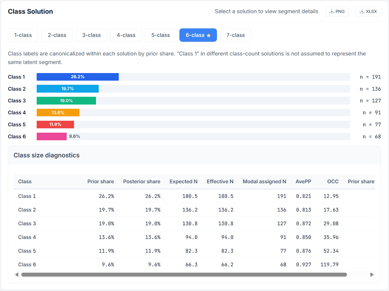
Figure 6. The 6-class solution of the Pizza run with the Class size diagnostics opened.
Below the pills, a horizontal bar chart shows each class’s share of the sample, with the modal count (n) next to each bar. The bar percentages are the average posterior class probabilities (posterior share). The a priori class sizes (prior share) appear in the Class size diagnostics table below the chart, together with their Wald interval.
The percentages sum to 100%. The n values are respondents assigned to the class by their largest membership probability; the posterior-weighted effective N appears in the tooltip.
An expandable Class size diagnostics table underneath the chart reports, per class:
Prior share: average model-implied class probability before observing a respondent’s choices.
Posterior share: average posterior class probability after observing choices.
Expected N: average prior share multiplied by respondent N.
Effective N: sum of posterior class probabilities across respondents.
Modal assigned N: count assigned to the maximum-posterior class.
AvePP: average posterior probability for respondents modally assigned to this class. Values around 0.80 to 0.90 indicate good class separation; values below 0.60 suggest fuzzy boundaries.
OCC: odds of correct classification relative to the class’s posterior-share odds.
Prior share 95% CI: Wald interval for the prior share, shown only when its standard error is available.
In the Pizza solution every class is well separated: AvePP lies between 0.81 and 0.93, and even the smallest class (9.6%) holds about 66 respondents, well above the minimum of 30. An XLSX link in the card header downloads the class shares and this diagnostics table for the selected solution.
4.4 Attribute Importances or MaxDiff Scores by Segment
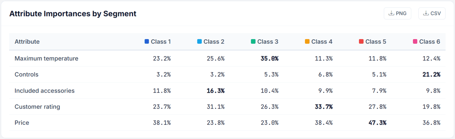
This table shows how important each attribute is for each segment. Importance is calculated as:
Attribute importance: the utility range of attribute a divided by the total utility range across all attributes.
Importances always sum to 100% within each class. The power of LC lies in revealing dramatically different importance profiles across segments:
Figure 7. Attribute importances of the 6-class Pizza solution. Bold marks the highest value in each row.
The six pizza oven segments differ clearly:
Class 3 (19%) is the only segment in which Maximum temperature leads (35.0%); price matters least here (23.0%).
Class 5 (12%) is the most price-driven segment (47.3%).
Classes 2 and 4 (20% and 14%) put Customer rating first or close to first (31.1% and 33.7%); Class 2 also gives the accessories the most weight (16.3%).
Class 6 (10%) is the only segment that cares about Controls (21.2% against 3 to 7% elsewhere).
Class 1 (26%) is price-led (38.1%) but still gives temperature and rating about a quarter each.
An aggregate model would average these patterns away. Who the people in each segment are is the subject of the next two cards.
Non-substantive terms are excluded from the importance calculation: the none-option ASC, the anchored MaxDiff threshold, and the CBC Shop display-position controls.
MaxDiff runs show scores, not importances
For MaxDiff and Anchored MaxDiff the card is titled Probability-Rescaled Scores by Segment and lists items instead of attributes. The scores are computed from the raw logit utilities as qi = exp(ui) / (exp(ui) + a − 1) and Scorei = 100 × qi / Σq, where a is the number of alternatives shown per MaxDiff set. Scores sum to 100% within each class. The formula is printed above the table.
For Anchored MaxDiff, the result overview also shows Anchored MaxDiff calibration included. Its item-vs-anchor observations restore absolute location information through a free threshold for each class; that threshold is part of estimation but is intentionally excluded from the item-score table.
4.5 Covariate Profile by Segment
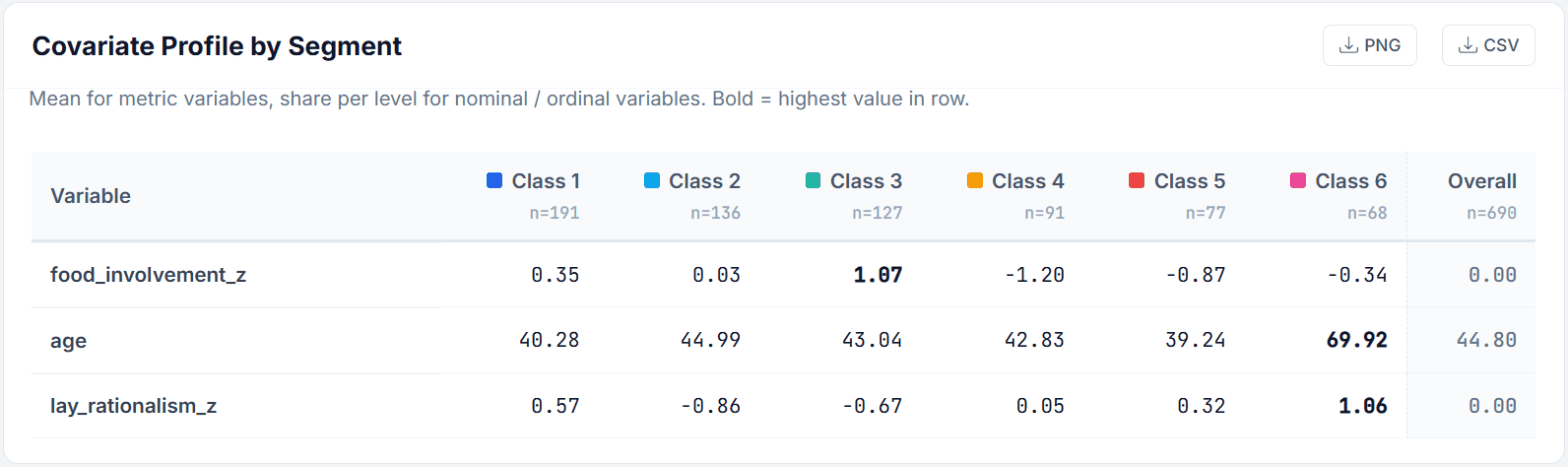
When you selected respondent covariates in either role, a Covariate Profile by Segment card describes the classes in the covariates’ own units: the mean for metric variables, and the share per level for nominal and ordinal variables. The highest value in each row is shown in bold, and an Overall column gives the full-sample value for comparison.
Figure 8. Covariate profile of the 6-class Pizza solution.
Read together with Figure 7, the segments get a face. The temperature-led Class 3 has by far the highest food involvement (+1.07 SD) and a low lay rationalism (−0.67 SD). Class 6, the segment that cares about the controls, is on average 70 years old and has the highest lay rationalism (+1.06 SD). The rating-led Class 4 and the price-driven Class 5 are clearly below average in food involvement (−1.20 and −0.87 SD).
How the numbers are computed
Profile values are posterior-weighted: for class c the metric mean is Σi wic xi / Σi wic and the categorical share is Σi wic 1[xi = level] / Σi wic, with wic the posterior membership probability. This is the Latent GOLD convention. The n under each class header is the modal count (respondents whose largest posterior probability is that class); the posterior-weighted effective N is in the header tooltip. The two therefore do not have to agree, and the modal counts do not have to sum exactly to the Overall n pattern.
4.6 BCH-Corrected Passive Profiles
For eligible standard LC runs with passive profiling variables, an additional BCH-Corrected Passive Profiles card applies a modified modal BCH correction, which adjusts the descriptive profile for classification error. It reports pairwise BCH-corrected Wald tests between classes, listing a pair when the Benjamini-Hochberg adjusted q-value is below 0.05.
The card states its own limits: HC0 respondent-clustered conditional sandwich intervals hold the fitted LC solution and the classification-error matrix fixed, so they do not include first-stage LC uncertainty.
When BCH is withheld
BCH profiling is not computed for concomitant LC (the posteriors already depend on active membership covariates) and not for respondent-weighted runs (the classification matrix and covariance do not yet support the survey design). In those cases the card explains the reason instead of showing numbers.
4.7 Raw and Zero-Centered Utilities
The full part-worth utilities for each attribute level within each class are the “DNA” of each segment, what each segment likes and dislikes. Choicery does not print them in the browser. The Raw and Zero-Centered Utilities card offers an XLSX download containing two formatted tables for the currently selected class solution:
Raw Utilities: the estimator parameters on the logit scale, as fitted.
ZCD Utilities: the presentation scale. Within each class, utilities are zero-centered within each attribute (the mean across levels is zero) and then rescaled by one class-specific factor so that the average utility range across the substantive attributes equals 100 (the none-option ASC, the anchored MaxDiff threshold and the CBC Shop display-position controls are scaled by the same factor but excluded from the target). Positive values mark preferred levels, negative values dispreferred levels. Standard errors in the XLSX are multiplied by the same factor; t and p refer to the raw-utility tests.
Switching the class solution pill in the Class Solution card updates this download link, so the XLSX always matches the solution you are looking at.
Scale confound warning
Do not compare raw utility magnitudes across classes. A utility of 2.5 in Class 1 does not mean the same as 2.5 in Class 2 because the response error (scale) differs across classes. Use attribute importances (range-normalized) for cross-class comparison. Within a single class, relative magnitudes and signs are always interpretable.
4.8 Class Membership Model (Concomitant LC only)
When Active membership covariates were selected during estimation (Section 3.3), an additional card appears: the Class Membership Model. It shows how each covariate affects the probability of belonging to each class.
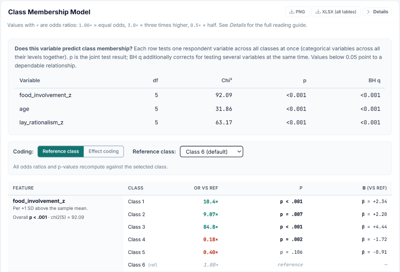
Figure 9. Class Membership Model of the 6-class Pizza solution (top part; the rows for age, lay_rationalism_z and the intercept follow below).
Values marked with × are odds ratios: 1.00× means equal odds, 3.0× three times higher, 0.5× half. A Details toggle in the card header opens the full reading guide, including which features were encoded and how.
Coding toggle
The coefficient table is long-format: one row per feature and class, with the columns Feature, Class, OR vs Ref, p and β (vs ref). The Feature cell spans that feature’s class rows and carries the omnibus result as “Overall p” plus the Chi² and df. A Coding control above the table offers two parameterizations, with a Reference class dropdown next to it:
Reference class (the default): each row is the odds ratio versus the selected base class, whose own row shows 1.00× and the p-value “reference”. All odds ratios and p-values recompute when you change the reference class.
Effect coding: the column headers change to OR vs grand mean and β (vs grand mean), so no class is the baseline and every class is treated symmetrically. Coefficients sum to zero across classes. Per-cell p-values require a joint test here, so the p cell reads “see Expert view”; judge the variable by the Overall p in the Feature cell instead. This matches the “Effects” parameterization used by Latent GOLD.
An expandable Expert view: raw coefficient matrix and tests at the bottom of the card holds the untransformed coefficient matrix.
Numeric standardized features are read as “one standard deviation above the sample mean”.
Does this variable predict class membership?
Above the coefficient table, a compact omnibus table answers exactly that question. Each row tests one respondent variable across all classes at once (categorical variables across all their levels together) and reports df, Chi², p, and BH q. The q-value additionally corrects for testing several variables at the same time. Values below 0.05 point to a dependable relationship.
Pizza example: reading the membership model
All three variables predict class membership (p and BH q below 0.001). Against the reference Class 6, one standard deviation more food involvement multiplies the odds of belonging to the temperature-led Class 3 by 84.8, while it lowers the odds for Class 4 (0.18×). Class 5 is not distinguishable from Class 6 on this variable (p = .106). For age every class shows odds ratios of about 0.004 to 0.006 against Class 6: one standard deviation older makes all other segments far less likely than the older Class 6. Such small or large odds ratios are typical when one segment is defined by a single variable; switch the Reference class to another class or use Effect coding to read the other contrasts.
P-values in this card come from a post-EM full-ML polish with an observed-information Hessian. When that could not be computed, the card says so and the coefficients are still shown as effect sizes.
The average prior shares (mean of πs(zi) across respondents) and average posterior shares (mean of his) are not repeated in this card; read them from the Prior share and Posterior share columns of the Class size diagnostics table (Section 4.3) or from the Membership Model sheet of the XLSX. An XLSX (all tables) link downloads the complete membership model: overview, covariate tests, coefficients versus reference, effect coding, all pairwise contrasts, and the raw coefficient matrix.
Actionable insight
The membership coefficients directly answer the question: “What kind of person is likely to be in each segment?” This enables predictive targeting, given a new customer’s demographic profile (but no choice data), you can estimate which segment they most likely belong to and tailor your offering accordingly.
4.9 Respondent Classification Uncertainty
Each respondent is assigned to their most probable class (the class with the highest posterior membership probability). The Respondent Classification Uncertainty card provides a CSV download with the complete per-respondent classification diagnostics, so you can inspect how confidently each person was placed.
This card is tied to the BIC-selected solution: it is hidden while you view a different class solution in the Class Solution switcher. In the Pizza example it is shown for the 6-class solution and disappears when you switch to 5-class.
For the aggregate view of the same question, use AvePP and OCC in the Class size diagnostics table (Section 4.3). Average posterior probabilities close to 1.0 mean the classes are well-separated. Values close to 1/S (for example 0.33 with three classes) mean the classes overlap substantially.
5. Saving Segments
Once you have identified a meaningful class solution, the Save Segments to Database card at the bottom of the Results step writes the segment assignments into your survey data for use in downstream analyses (market simulation, filtering, exports).
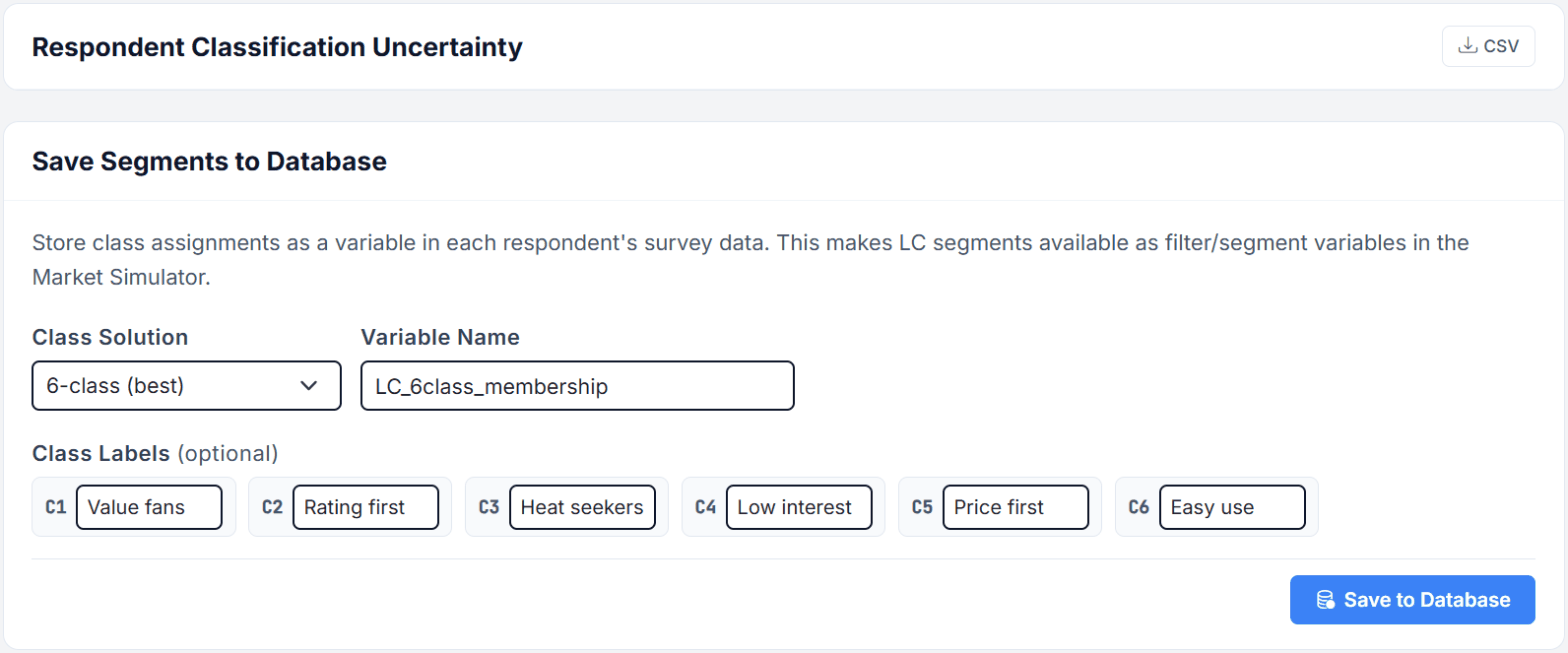
Figure 10. Saving the 6-class Pizza solution with descriptive class labels; above it the Respondent Classification Uncertainty card of section 4.9.
1
Pick the Class Solution from the dropdown. It starts on the BIC-selected solution (“6-class (best)” in the Pizza run), independent of the pill you selected above, so check that it is the solution you want to report. You can only save one solution at a time, but you can save multiple solutions under different variable names.
2
Enter a Variable Name. Choicery pre-fills LC_<best>class_membership, for example LC_3class_membership. The name must start with a letter or underscore and may then contain letters, digits and underscores, up to 60 characters. It appears as a new column in your survey data.
3
Optionally fill in the Class Labels. One input appears per class of the selected solution, pre-filled with the class number. Replace the numbers with short descriptive names based on the importances and profiles, for example “Heat seekers” for the temperature-led Class 3 of the Pizza solution.
4
Click “Save to Database.” Choicery stores the class assignments as a variable in each respondent’s survey data. Saved segments become available as filter and segment variables in the Market Simulator and in data exports.
Naming segments
Good segment names summarize the “essence” of each class in 2 to 3 words. Look at attribute importances and the dominant utility patterns. Examples: “Budget Shoppers,” “Tech Enthusiasts,” “Premium Brand Seekers,” “Feature Maximizers.”
6. Exporting Results
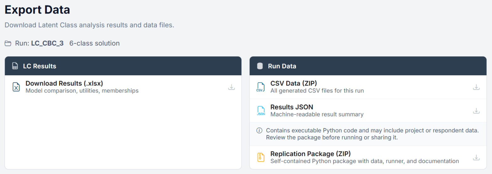
Step 3 Export lists four downloads for the active run, grouped into two cards, LC Results and Run Data. The line above the cards names the run and its BIC-selected solution; the workbook still contains one sheet per class solution.
Figure 11. The Export step of the Pizza run.
Download
Contents
Use Case
Download Results (.xlsx)
Multi-sheet workbook: summary, settings summary, one sheet per class solution with importances and utilities, segment membership, and, where applicable, membership model, membership significance, covariate profile and BCH profiles
Sharing results with stakeholders, further analysis in Excel
CSV Data (ZIP)
All CSV files generated for this run, including Model_Comparison.csv and, per class solution, Class_Betas.csv, Class_Betas_Raw.csv, Class_Betas_Inference.csv, Class_Sizes.csv, Class_Memberships.csv, Class_Profiles.csv and the membership tables
Import into R, Python, or other statistical software
Results JSON
Machine-readable result summary with model parameters and fit statistics
API integration, custom reporting scripts
Replication Package (ZIP)
Self-contained Python package with data, runner and documentation
Complete audit trail and reproducibility
The Replication Package carries a notice in the UI: it contains executable Python code and may include project or respondent data, so review it before running or sharing it. Depending on your project it can also be shown as locked, with the reason displayed in place of the description.
Class_Betas_Inference.csv
This tidy long-format file carries the class-specific part-worth utilities together with their standard errors, t-values and p-values, one row per class and level. It is the file to use when you need to report whether a segment’s preference for a level is statistically distinguishable from zero.
Result cards in the Results step carry their own targeted exports as well: PNG and CSV buttons on Model Comparison, Attribute Importances by Segment and Covariate Profile by Segment; PNG plus an XLSX link on Class Solution; a CSV button on BCH-Corrected Passive Profiles; an XLSX link on Raw and Zero-Centered Utilities; PNG plus XLSX (all tables) on Class Membership Model; and a CSV link on Respondent Classification Uncertainty. A Download PDF button sits in the Results header for supported task types.
7. Best Practices & Common Pitfalls
Do:
Start with a wide range (Min 2, Max 8 to 10) and let BIC guide the choice. The 1-class pooled MNL baseline is added automatically, so you always get a reference point.
Use multiple random starts (≥5) to avoid local optima. The EM algorithm is not guaranteed to find the global maximum, different starting values can lead to different solutions.
Profile segments with demographics to make them actionable. A segment is only useful if you can identify and reach its members.
Look at segment sizes. Very small segments (<5% of the sample) may represent noise rather than a genuine subgroup.
Compare results across different random seeds for stability. If a 3-class solution looks very different with seed=1 vs. seed=42, the solution is unstable and the data may not support 3 classes reliably.
Name your segments based on their utility profiles. Generic labels like “Class 1” are meaningless to stakeholders.
Check the “Ready to Report?” column. Always verify that your chosen model shows Yes. A No means it did not converge, failed the stricter final stability and identification checks, or has an expected smallest class below 30 respondents; its parameter estimates may still move or rest on too few people.
Don’t:
Don’t force a specific number of classes based on prior expectations alone. Let the data speak, you might expect 4 segments but BIC might say 3 is optimal.
Don’t compare raw utility magnitudes across classes (scale confound). Use importances instead. A utility of 3.0 in Class 1 and 1.5 in Class 2 does not mean Class 1 cares “twice as much”, the scales are not comparable.
Don’t ignore a “provisional” warning in the Solution diagnostics box. Increase Max EM Iterations, tighten LL Tolerance, and rerun. If it persists, report the lowest-BIC model among the rows marked Yes under Ready to Report.
Don’t use LC for individual-level prediction. LC assigns each person to a segment, but within each segment everyone gets the same utilities. For individual-level preferences, use HB estimation.
Don’t assume segment membership is binary. It’s probabilistic, a respondent might have 70% probability of belonging to Class 1 and 30% to Class 2. Treating assignments as certain when posterior probabilities are low can be misleading.
Don’t over-extract. More classes does not always mean a better model. Each additional class adds parameters and increases the risk of overfitting, especially with small samples.
The local optima trap
The EM algorithm can get stuck in local optima, solutions that are locally best but not globally optimal. Always use multiple random starts. If you run with only 1 start and get a poor solution, increasing to 10 to 20 starts often reveals a substantially better model (higher log-likelihood, more interpretable segments).
Part II
Theoretical Background
The statistical foundations behind Latent Class MNL estimation, for researchers and advanced users.
8. Key Definitions
Glossary
Latent Class
An unobserved (hidden) discrete subgroup within a population. Members of the same class share similar preferences but differ from members of other classes.
Finite Mixture Model
A statistical model that assumes the observed data comes from a mixture of a finite number of component distributions. LC-MNL is a finite mixture of multinomial logit models.
EM Algorithm
Expectation-Maximization, an iterative algorithm for fitting mixture models. Alternates between computing expected class memberships (E-step) and re-estimating model parameters (M-step) until convergence.
Class Membership Probability
The posterior probability that respondent i belongs to class s, given their observed choices. Computed using Bayes’ theorem after model estimation.
BIC (Bayesian Information Criterion)
A model selection criterion that balances fit (log-likelihood) against complexity (number of parameters). BIC = −2·LL + k·ln(N), where N is the number of unweighted likelihood components (observed choices plus, for Anchored MaxDiff, anchor answers), not the respondent count. Lower is better.
AIC (Akaike Information Criterion)
A model selection criterion with less complexity penalty than BIC. AIC = −2·LL + 2k. Tends to select more complex models than BIC.
CAIC (Consistent AIC)
A variant of AIC proposed by Bozdogan (1987) that adds a stronger complexity penalty. CAIC = −2·LL + k·(ln(N) + 1), with the same N convention as BIC.
Zero-Centered Diffs
Part-worth utilities rescaled so that the mean across levels within each attribute is zero. This is the standard representation in conjoint analysis, making it easy to see which levels are preferred (positive) and dispreferred (negative).
Pct Certainty
A goodness-of-fit measure: (LLmodel − LLnull) / (−LLnull) × 100%. Also known as McFadden’s pseudo-R². Values of 0.2 to 0.4 are considered good for discrete choice models.
Effects Coding
A coding scheme for categorical variables where the omitted level is coded as −1 (not 0 as in dummy coding). This produces part-worth utilities that are zero-centered within each attribute.
9. The LC-MNL Model
9.1 Core Model
The Latent Class Multinomial Logit (LC-MNL) model assumes that the population consists of S distinct classes, each with its own set of preference parameters. The unconditional choice probability is a finite mixture:
P(j chosen) = Σs=1S αs · Ps(j)
Mixture model: the overall choice probability is a weighted average across classes.
where:
αs = the a priori class membership probability (class size), with Σs αs = 1
Ps(j) = the MNL choice probability for alternative j within class s
Within each class, choices follow a standard Multinomial Logit (MNL) model:
Ps(j) = exp(Vjs) / Σk exp(Vks)
Within-class MNL probability. Vjs is the systematic utility of alternative j in class s.
The systematic utility is a linear function of attribute levels:
Vjs = Σa βas · xja
Linear-in-parameters utility. βas are class-specific part-worth utilities; xja are attribute level indicators.
The full likelihood of the model, across all respondents i and all choice tasks t, is:
L = Πi Σs αs · Πt Ps(yit | xit, βs)
Full likelihood. Product over respondents i, sum over classes s, product over choice tasks t. yit is the observed choice.
This expression says: for each respondent, sum over all possible class memberships (weighted by class sizes), and within each class, multiply the MNL probabilities of all observed choices. The key insight is that the summation is inside the product over respondents, class membership is unknown and must be integrated out.
Intuition
Imagine each respondent flips a weighted coin to join one of S classes (weights = αs). Once in a class, they make choices according to that class’s MNL model. We observe the choices but not the coin flip. The EM algorithm figures out the most likely “coins” (class sizes) and “utility weights” (betas) that explain the observed choices.
9.2 Posterior Class Membership
After estimating the model, we can compute the posterior probability that respondent i belongs to class s, given their observed choices:
Bayes’ theorem applied to class membership. The numerator is the joint probability of class s and the observed choices; the denominator normalizes across all classes.
This is a direct application of Bayes’ theorem:
Prior: αs, the overall probability of being in class s
Likelihood: Πt Ps(yit), how likely are respondent i’s observed choices under class s’s preferences?
Posterior: P(s | yi), the updated probability after seeing the data
A respondent whose choices are very consistent with Class 2’s preferences will receive a high posterior for Class 2 and low posteriors for other classes. A respondent whose choices are equally consistent with multiple classes will have more diffuse posteriors.
10. The EM Algorithm
10.1 Overview
The LC-MNL model cannot be estimated in closed form because the class membership is unobserved. The Expectation-Maximization (EM) algorithm is the standard approach. It iterates between two steps:
E
E-step (Expectation): Given the current parameter estimates (βs, αs), compute each respondent’s posterior membership probabilities P(s | yi) using Bayes’ theorem (Section 9.2). These are the “expected” class memberships.
M
M-step (Maximization): Re-estimate the model parameters. For each class s, estimate βs by running a weighted MNL estimation where respondent i’s observations are weighted by P(s | yi). Update the class sizes as αs = (1/N) Σi P(s | yi).
The algorithm iterates E → M → E → M → ... until the log-likelihood converges (i.e., the improvement between iterations falls below a tolerance threshold). The EM algorithm is guaranteed to increase the log-likelihood at every iteration (or leave it unchanged), but it is not guaranteed to find the global maximum.
LL = Σi log [ Σs αs · Πt Ps(yit | xit, βs) ]
Log-likelihood function. The EM algorithm maximizes this by alternating E-steps and M-steps.
10.2 Choicery Implementation Details
Choicery’s LC estimation uses the following implementation choices:
M-step optimization: L-BFGS-B (a bounded quasi-Newton method) with an analytic gradient, one class at a time, each capped at 20 optimizer iterations with ftol 1e-6 per EM iteration (a generalized EM: the M-step improves rather than fully maximizes the weighted MNL likelihood). An update that would worsen the class objective is rejected and counted; any rejected update fails the final reliability check.
Sign constraints: Sign constraints on linear attributes are implemented as coefficient bounds passed to L-BFGS-B, not as a penalty.
Ridge regularization: The within-class utility M-step runs unregularized. A small L2 ridge (1e-6) is applied to the membership coefficients of the concomitant model for numerical stability, which prevents degenerate solutions when classes have very few effective observations.
Multiple random starts: The full EM algorithm is run from N different random starting points. Only the solution with the highest final log-likelihood is retained; the number of starts that met the stopping rule is reported as EM Starts.
Adaptive continuation: If the highest-likelihood start stops at the Max EM Iterations cap without meeting the stopping rule, Choicery does not discard it. It continues that exact parameter state for up to two further rounds of Max EM Iterations each and stops early when the round converges or improves the log-likelihood by less than the LL Tolerance. A start that converges during continuation counts toward EM Starts. If it still has not converged, the solution is kept as the best fit found but flagged provisional.
Convergence criterion: The EM stops when the absolute improvement in log-likelihood is less than the tolerance (default: 0.001).
Final reliability check: Meeting the EM stopping rule is not sufficient for the “Ready to Report” flag. After the EM finishes, Choicery evaluates the observed-data score norm at the reported parameters, normalized per model observation, against a limit of 1e-3 per observation. The gate additionally requires no likelihood decrease during the EM, no rejected optimizer update, and, for concomitant runs, a successful full-ML polish. When a sign-constraint bound is active the score is legitimately non-zero at the boundary, so Choicery falls back to a last-step parameter-movement limit (1e-3) instead. The limit is calibrated empirically: EM solutions stopped at the default LL tolerance sit around 1e-4 per observation on real data, while genuinely unconverged fits sit at 1e-2 and above.
Class size constraints: Class sizes (αs) are constrained to be positive and sum to 1. The Solution diagnostics box shows “Possible separation or a degenerate class” when any class part-worth or membership coefficient reaches an absolute value of 20 or the smallest prior share falls to 0.01% or below. Independently, Choicery flags a solution as not ready for reporting when its smallest expected class is below 30 respondents (Section 4.2). As a rule of thumb, treat a BIC-selected model whose smallest class holds less than 5% of respondents, or in which fewer than half of the class part-worths are significant at the 5% level, as possibly over-specified and compare it with the next smaller model.
Standard errors: Class part-worth standard errors, t-values and p-values are computed from an observed-information Hessian (forward differences of the analytic gradient) and exported in Class_Betas_Inference.csv. Wald inference is withheld when the model has more than 220 free parameters, when a sign constraint is active at its bound, or when respondent weights are used; the Utility inference row of the Solution diagnostics box then reads Withheld. A 1-class fit is mathematically identical to an aggregate MNL, which makes it a useful sanity check.
10.3 Random Starts
The EM algorithm is sensitive to initialization. Different starting values for βs and αs can lead to different solutions (local optima). This is a fundamental property of mixture models, not a bug.
Why random starts matter
With a single start, you might find a “local optimum”, a solution that is better than nearby solutions but not the best overall. Multiple starts explore different regions of the parameter space. The best solution (highest LL) across all starts is much more likely to be the global optimum.
Choicery runs the full EM from N different random starting points and keeps the solution with the highest log-likelihood. Practical recommendations:
Use Case
Random Starts
Notes
Quick exploration
3 to 5
Fast, but may miss the global optimum for complex models
Standard analysis
5 to 10
Good balance of speed and reliability
Publication / final results
10 to 20
High confidence in finding the global optimum
Complex models (≥6 classes)
20 to 50
More classes = more local optima = more starts needed
11. Model Selection, Information Criteria
The central question in LC analysis is: how many classes? More classes always improve the log-likelihood (better fit), but at the cost of more parameters (more complexity). Information criteria balance fit against complexity.
The Three Criteria
AIC = −2 · LL + 2k
Akaike Information Criterion (Akaike, 1974). k = number of free parameters.
BIC = −2 · LL + k · ln(N)
Bayesian Information Criterion (Schwarz, 1978). N is the number of unweighted likelihood components: observed choices plus, for Anchored MaxDiff, anchor answers; Best and Worst answers each count once. Choicery does not use the respondent count here (no respondent-level panel BIC), and the Results step prints the N it used below the meta bar. Penalizes complexity more than AIC.
CAIC = −2 · LL + k · (ln(N) + 1)
Consistent AIC (Bozdogan, 1987), same N convention as BIC. Penalizes complexity even more than BIC.
AIC3 = −2 · LL + 3k
Modified AIC with a penalty of 3 per parameter (Bozdogan, 1994); often recommended for mixture models. Reported in the Model Comparison CSV and the XLSX.
ABIC = −2 · LL + k · ln((N + 2) / 24)
Sample-size-adjusted BIC (Sclove, 1987) with the same N convention as BIC. Reported in the Model Comparison CSV and the XLSX.
Number of Free Parameters
For an LC-MNL model with C classes and P parameters per class (the number of utility coefficients):
k = C · P + (C − 1)
Total free parameters. C · P for the class-specific betas, plus C − 1 for the class size parameters (the last α is determined by the sum-to-one constraint).
Pizza example: Parameter Count
Design: Maximum temperature (3 levels), Controls (3), Included accessories (3),
Customer rating (4) categorical, Price linear, plus the none option
Parameters per class: 2 + 2 + 2 + 3 + 1 + 1 (NoneOpt) = 11
Standard 6-class model:
k = 6 × 11 + (6-1) = 66 + 5 = 71 parameters
How to Choose
BIC is the most commonly used criterion in applied conjoint research and Choicery’s default. It penalizes complexity more heavily than AIC, tending to select more parsimonious (fewer classes) models.
AIC may select more classes than BIC. Some researchers report both and note any discrepancies.
CAIC is the most conservative, it will never select more classes than BIC.
A useful visual approach is the “elbow plot”: plot BIC (y-axis) against the number of classes (x-axis). The optimal number of classes is where the curve “bends”, where adding more classes no longer substantially reduces BIC.
The curve drops steeply up to 4 classes and is almost flat from 4 to 6: the 5-class and 6-class models differ by only 4.4 BIC points, and 7 classes are worse again. The 6-class model is selected; with a gap this small, interpretability decides whether the sixth class is worth keeping (section 4.2).
BIC is a guide, not a law
Information criteria provide valuable guidance, but should not be followed blindly. Always consider interpretability (do the segments make substantive sense?), stability (do they replicate across random seeds?), and actionability (can you do something different for each segment?). A solution with one more or fewer class than the BIC optimum may be preferable on these grounds.
12. Interpreting and Comparing Segments
12.1 The Scale Factor Problem
A fundamental property of discrete choice models is that the scale of the utility function is not identified, only ratios of utilities are meaningful. In LC-MNL, each class has its own scale factor, which is confounded with the magnitude of the betas.
Concretely: if Class 1 has betas that are twice as large as Class 2’s, this does not mean Class 1’s preferences are “twice as strong.” It may simply mean that Class 1 respondents are more consistent (lower response error = higher scale), which inflates all utility magnitudes proportionally.
Practical implication
Never compare raw utility values across classes. A beta of 3.0 in Class 1 is not “bigger” than a beta of 1.5 in Class 2 in any meaningful sense. Instead, use attribute importances (utility range as a percentage of total range), which are scale-free and can be compared across classes.
Within a single class, relative magnitudes are meaningful: if Brand A has a utility of 2.0 and Brand B has 1.0 (both in Class 1), then Class 1 genuinely prefers Brand A over Brand B, and the preference is twice as large as the Brand B preference (relative to the zero point).
13. Concomitant LC-MNL: Covariate-Driven Class Membership
13.1 Motivation
Standard LC-MNL treats the class membership probabilities αs as constants, every respondent has the same a priori probability of belonging to each class, regardless of their demographics or attitudes.
This raises a natural question: if we know that age, income, or attitudes are related to segment membership, why not incorporate that information during estimation?
Concomitant LC-MNL (also called Latent Class Regression or LC with covariates) does exactly this. It replaces the constant class sizes with respondent-specific class membership probabilities that depend on observed covariates (DeSarbo, Wedel, Vriens & De Sarbo, 1992; Wedel & Kamakura, 2000).
The key idea
Instead of “45% of respondents are in Segment 1,” the model says “younger, lower-income respondents have a 65% probability of being in Segment 1, while older, higher-income respondents have only a 25% probability.” Class membership becomes a function of who the respondent is, not a single number for the whole sample.
13.2 The Concomitant Model
In the standard LC-MNL (Section 9), the unconditional choice probability is:
P(j chosen by i) = Σs αs · Ps(j | βs)
Standard LC: constant class sizes αs for all respondents.
In the concomitant extension, the constant αs is replaced by a respondent-specific probability πs(zi):
P(j chosen by i) = Σs πs(zi) · Ps(j | βs)
Concomitant LC: class membership depends on respondent covariates zi.
The class membership probabilities are modeled as a multinomial logit over respondent covariates:
πs(zi) = exp(γs′ zi) / Σs′ exp(γs′′ zi)
Membership MNL. γs is a vector of coefficients for class s. zi includes an intercept and respondent covariates (demographics, attitudes).
For identification, one class is designated as the reference class with γ fixed to zero. The γ coefficients for the other classes represent log-odds of belonging to that class relative to the reference class.
13.3 How It Changes the EM Algorithm
The EM algorithm (Section 10) is modified in two places:
E
E-step: Instead of using constant log(αs) for all respondents, use respondent-specific log(πs(zi)). The posterior computation otherwise remains the same.
M
M-step (class sizes): Instead of αs = mean(posteriors), estimate the γ coefficients by fitting a weighted multinomial logit where the posterior class probabilities serve as soft labels. The class-specific utility parameters βs are updated exactly as before.
The γ-estimation in the M-step is itself a standard MNL optimization. It uses the same L-BFGS-B optimizer already employed for the within-class betas, with a well-known closed-form gradient:
∂L / ∂γs = Σi (his − πs(zi)) · zi
Gradient for membership coefficients. his is the posterior probability from the E-step, πs(zi) is the current membership prediction.
Choicery implementation note. After the EM has finished for every class count, each concomitant solution is polished by a direct full-maximum-likelihood step that optimizes all class part-worths and membership coefficients jointly with L-BFGS-B (at most 500 iterations; it stops earlier once the relative improvement falls below ftol 1e-9). The polished parameters and log-likelihood replace the EM values, the information criteria are recomputed, the best model is re-selected by BIC, and the observed-information Hessian for the p-values in the Class Membership Model card is taken at the polished solution. A failed polish marks the solution as not ready for reporting.
13.4 Parameter Count
The number of free parameters changes because the membership model adds coefficients:
k = C · P + (C − 1) · K
C = number of classes, P = utility parameters per class, K = number of encoded membership features (including intercept). Compare to standard LC where k = C · P + (C − 1).
Pizza example: Parameter Count Comparison
Design: 11 utility parameters per class (see section 11)
3 active membership covariates (food_involvement_z, lay_rationalism_z, age)
→ Encoded features K = 4 (intercept + 3 standardized covariates)
Standard 6-class: k = 6 × 11 + (6-1) = 71 parameters
Concomitant 6-class: k = 6 × 11 + (6-1) × 4 = 86 parameters
The concomitant model has 15 additional parameters (5 non-reference classes × 3 covariates), which gives the 86 shown in the Model Comparison of the Pizza run. BIC charges for them, so covariates only pay off when they genuinely improve fit.
When does concomitant LC help?
Concomitant LC improves model fit only when covariates are genuinely predictive of class membership. If demographics have no relationship with preference segments, the additional parameters add noise without improving fit, and BIC will correctly penalize the concomitant model. In practice, 3 to 5 well-chosen covariates work best. Too many covariates relative to sample size can cause estimation instability.
13.5 Interpretation of γ Coefficients
The γ coefficients have a clear interpretation as log-odds ratios:
Positive γs,d: higher values of covariate d increase the odds of belonging to class s (relative to the reference class).
Negative γs,d: higher values of covariate d decrease the odds of belonging to class s.
γ = 0: the covariate has no effect on membership in that class (or it is the reference class).
Example: Interpreting Membership Coefficients
Covariate
Class 1 (γ)
Class 2 (γ)
Class 3 (ref)
Intercept
0.82
−0.34
0.00
Age (z-scored)
−0.45
0.31
0.00
Income (high)
−0.62
0.48
0.00
Interpretation: Younger, lower-income respondents are more likely to be in Class 1 (the price-sensitive segment). Older, higher-income respondents are more likely to be in Class 2 (the brand-loyal segment). Class 3 is the reference, respondents with “average” demographics have roughly equal odds for all classes (depending on the intercept).
13.6 Prior vs. Posterior Probabilities
It is important to distinguish two types of respondent-level probabilities in concomitant LC:
Probability
Definition
Depends On
Use
Prior πs(zi)
Probability of class membership based on covariates alone
Demographics, attitudes
Understanding who tends to be in each class
Posterior his
Updated probability after observing the respondent’s choices
Covariates + choice data
Class assignments, saving segments
The posterior is always more informative than the prior: it incorporates both who the respondent is (covariates) and how they actually chose (choice data). Class assignments in Choicery are always based on the posterior, as in standard LC.
13.7 Why Concomitant LC Instead of Post Hoc Analysis
Concomitant LC incorporates covariates during estimation, which is statistically superior to analyzing demographics after the fact. Post hoc profiling (cross-tabulating demographics with hard class assignments) has two weaknesses: (1) segments are formed without considering covariate information, and (2) significance tests are optimistic because class assignments are themselves estimated from data.
With concomitant LC, covariates directly influence segment formation, which can sharpen class separation when covariates are truly predictive. It also enables predicting segment membership for new respondents based on their demographic profile alone, without requiring choice data.
14. LC vs. HB, When to Use Which
Latent Class (LC) and Hierarchical Bayes (HB) are the two dominant methods for capturing preference heterogeneity in conjoint analysis. They are complementary, not competing methods (Orme & Chrzan, 2017).
Goal
LC-MNL
HB
Market segmentation
Best choice, produces discrete, actionable segments with distinct preference profiles directly.
Not designed for segmentation. Requires post-hoc clustering of individual utilities (K-means, etc.).
Individual-level utilities
Not ideal, within each class, all members share the same utilities. No individual variation captured.
Best choice, produces individual-level part-worths for every respondent.
Sparse data (few tasks per respondent)
Better stability, fewer parameters per respondent (just class membership).
May overfit with too few observations per respondent.
Continuous heterogeneity
Cannot model, assumes within-class homogeneity. Heterogeneity is captured only across classes.
Models continuous distributions (multivariate normal) of preferences.
Named segments for management
Direct output, each class has a clear profile that can be named and communicated.
Requires post-hoc analysis (clustering) to derive named segments.
Market simulation
Not run on class utilities in Choicery. Save the class assignments (Section 5) and use them as a segment or filter variable in the HB-based Market Simulator to compare segments.
The Market Simulator runs on individual-level HB utilities, the gold standard for aggregate share predictions.
Computational cost
Fast (seconds to minutes). EM converges quickly.
Slower (MCMC with thousands of iterations). Minutes to hours.
Best practice: use both
In a typical conjoint project, run HB first for individual-level utilities and market simulation, then run LC for segmentation and strategic insights. The two analyses answer different questions and together provide a complete picture of the market.
When LC Shines
When the business question is “How many types of customers do we have?” or “What are the key segments?”
When you need segments that can be directly communicated to management (“40% of the market is price-sensitive”)
When sample sizes are small and HB individual-level estimates would be noisy
When you want to understand the structure of heterogeneity (discrete types vs. continuous variation)
When HB Shines
When you need individual-level predictions (e.g., for targeted marketing or personalization)
When running market simulations that require realistic heterogeneity
When preference heterogeneity is truly continuous (no discrete “types”)
When you have enough data per respondent (8+ choice tasks) for stable individual estimates
15. Willingness to Pay by Segment
The results page shows a money value for each segment. It uses the ratio method on the raw class utilities: the utility difference between a level and its comparison level, divided by the utility change per money unit. Nothing about the estimation changes. A different price attribute or direction recalculates the table without a new run.
Choicery preselects the attribute whose name looks like a price, or else the only attribute whose levels carry a currency. Otherwise you choose it. Choose “(None - no price attribute)” if the study has none. The setting is separate from the Market Simulator. The direction starts at “Lower is better (price)”. For a value such as salary, choose “Higher is better (e.g. salary)”: a positive value is then the salary a person can give up for the improvement.
The 95% interval is a Fieller interval for that row. It uses the covariance of the class utilities from the estimation.
Negative values with “prefers higher prices”: this class chooses higher prices more often, so an improvement gets a negative value.
“barely reacts”, no value: the utility changes by 0.1 or less over the whole money range, so the ratio would be arbitrarily large.
“no finite interval”: the money coefficient cannot be told apart from zero, so the data give no upper or lower limit.
No interval at all: the estimation has no usable covariance, for example with respondent weights or an estimated Worst scale. The page names the reason.
The share-weighted average appears only when every class has a normal value. It has no interval.
16. References
Bozdogan, H. (1987). Model selection and Akaike’s Information Criterion (AIC): The general theory and its analytical extensions. Psychometrika, 52(3), 345-370.
DeSarbo, W. S., Ramaswamy, V., & Cohen, S. H. (1995). Market segmentation with choice-based conjoint analysis. Marketing Letters, 6(2), 137-147.
DeSarbo, W. S., Wedel, M., Vriens, M., & De Sarbo, C. (1992). Latent class metric conjoint analysis. Marketing Letters, 3(3), 273-288.
McLachlan, G. J., & Peel, D. (2000). Finite mixture models. New York: Wiley.
Orme, B. K. (2020). Getting started with conjoint analysis: Strategies for product design and pricing research (4th ed.). Manhattan Beach, CA: Research Publishers LLC.
Orme, B. K., & Chrzan, K. (2017). Becoming an expert in conjoint analysis: Choice modeling for pros. Orem, UT: external conjoint software.
Rao, V. R. (2014). Applied conjoint analysis. Berlin: Springer.
Schwarz, G. (1978). Estimating the dimension of a model. Annals of Statistics, 6(2), 461-464.
Vriens, M., Wedel, M., & Wilms, T. (1996). Choice-based conjoint analysis and market segmentation. Marketing Letters, 7(3), 245-256.
Vermunt, J. K., & Magidson, J. (2005). Technical guide for Latent GOLD 4.0: Basic and advanced. Belmont, MA: Statistical Innovations Inc.
Wedel, M., & Kamakura, W. A. (2000). Market segmentation: Conceptual and methodological foundations (2nd ed.). Boston: Kluwer Academic Publishers.