How to estimate individual-level preferences with Hierarchical Bayes (HB): every setting of the estimation form, how to read the results, and the method behind it. Worked example: the pizza oven CBC of the Pizza (Example) study.
Everything you need to run, interpret, and export HB analyses in Choicery.
1. What Is HB Estimation?
Hierarchical Bayes (HB) estimation discovers each individual respondent’s preferences from their choice data. Unlike aggregate models that estimate one set of preferences for everyone, HB produces a unique preference profile for every respondent in your study.
The key trick is called “borrowing strength.” HB uses information from all respondents to improve the estimates for each respondent. A respondent who answered only 10 choice tasks gets better estimates because HB knows what the overall population looks like. Respondents with noisy or sparse data are “pulled” toward the population average (a phenomenon called shrinkage), while respondents with clear, consistent choice patterns retain their individual signal.
The core idea
Imagine estimating each respondent’s preferences in isolation, with only 10 choice tasks. You would get very noisy estimates. Now imagine also knowing what the typical respondent looks like (from the full sample of several hundred people). HB combines both sources of information: each respondent’s own data plus the population distribution. The result is much better individual-level estimates than you could get from either source alone.
Key Output
Individual-level part-worth utilities: preference weights for every attribute level, for every respondent. These are the foundation for market simulation, WTP analysis, and segmentation.
Population-level parameters: the mean vector and covariance matrix of the multivariate normal distribution of preferences across respondents.
Model fit diagnostics: R-hat, ESS, RLH, hit rates, and other convergence and prediction quality metrics.
Why HB Is the Industry Standard
HB has been the dominant estimation method for conjoint analysis since the early 2000s. It is used by commercial conjoint software, Choicery, and throughout academic research (Rossi, Allenby, & McCulloch, 2005). Its popularity stems from three advantages:
Individual-level estimates enable respondent-level simulation, WTP, and clustering.
Borrowing strength produces stable estimates even with modest sample sizes or task counts.
Flexible heterogeneity: the multivariate normal population distribution captures correlations between preferences (e.g., people who prefer a high oven temperature also tend to care more about the accessories).
HB vs. Latent Class
HB and Latent Class (LC) are complementary, not competing. HB gives you continuous, individual-level estimates, ideal for simulation and WTP. LC gives you discrete segments, ideal for segmentation strategy. Best practice: run both. Use HB utilities for simulation; use LC for segment discovery and targeting.
2. Prerequisites
1
A conjoint task with collected responses. HB works with all conjoint types supported by Choicery: CBC, CBC Shop, DR-CBC, BW-CBC, MaxDiff, and Anchored MaxDiff. The conjoint task and its experimental design must already exist in your project.
2
At least ~50 respondents. HB can technically run with fewer, but results become unreliable below 50. For commercial studies, 200+ respondents are typical. More respondents means a better-estimated population distribution, which in turn improves every individual’s estimates through borrowing strength.
3
Open the Conjoint Analysis page. In the header menu choose Analysis → Conjoint Analysis. Pick your task in the sidebar under Analysis Tasks and stay on the first tab, Preference Analysis (HB). The other tabs are AI-Driven Profile Analysis, Latent Class and Interaction Effects (greyed out where a task type does not support them; Interaction Effects says "Conjoint only" on MaxDiff tasks). Below the tabs sits the three-step strip Estimation → Results → Export, with the participant-filter button on the left and the Methodology Guide link (this guide) on the right.
Sample size guidance
While HB is robust with small samples (thanks to borrowing strength), the population-level parameters become poorly estimated below ~50 respondents. With fewer than 30 respondents, collect more data before you rely on the results. For complex designs with many attributes or levels, aim for 200+ respondents.
3. Running HB in Choicery
3.1 The Estimation Form
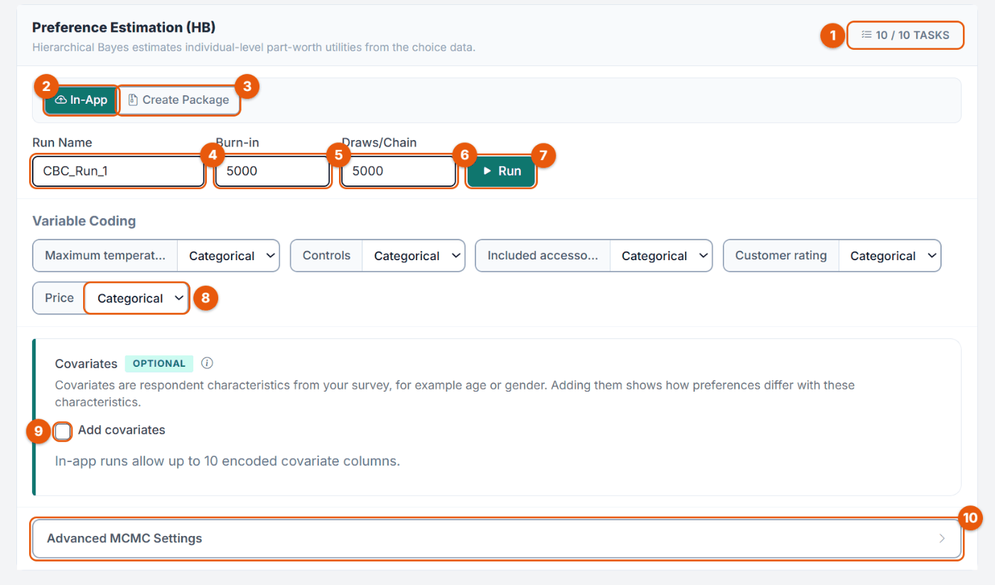
Each HB estimation is stored as a named run. You can keep up to 10 saved runs per conjoint task with different settings and compare them; only one estimation per user runs or waits in the queue at a time. Figure 1 shows the form of the Pizza oven CBC (cbc_pizza_oven, 690 respondents).
Figure 1. The estimation form (Pizza task cbc_pizza_oven).
No.
Control
What it does
1
Tasks badge
How many choice tasks enter estimation after the Choice Tasks filter and a random holdout task (here 10 / 10). Fixed tasks are kept out for holdout validation.
2
In-App
Runs the estimation on the Choicery server (default). Results appear in Results by themselves.
3
Create Package
Builds a Julia package you run on your own computer and import afterwards (section 3.3). Pro and Enterprise plans; on Free the pill opens the upgrade dialog.
4
Run Name
Up to 50 characters, required. The suggestion depends on the task type: CBC_Run_1, SCBC_Run_1 (CBC Shop), DRCBC_Run_1, BWCBC_Run_1, MD_Run_1 (MaxDiff), AMD_Run_1 (Anchored MaxDiff).
5
Burn-in
Iterations discarded at the start, while the sampler settles (default 10,000, steps of 100).
6
Draws/Chain
Iterations kept after burn-in (default 10,000). Draws divided by Thinning must leave at least 100 stored draws per chain, so with the default Thinning of 5 the minimum is 500.
7
Run
Starts the estimation. In Create Package mode it reads Generate Package.
8
Variable Coding
Categorical or Linear per attribute (section 3.5).
9
Add covariates
Adds respondent characteristics as a second model layer (section 3.4).
10
Advanced MCMC Settings
Opens the sampler, validation and reproducibility settings (section 3.7).
In-app runs have a budget of 100,000 iterations per chain for Burn-in plus Draws together. A larger total is refused when you click Run ("Burn-in plus draws per chain must not exceed 100,000 for an in-app run.").
How many iterations do you need?
The defaults (5,000 + 5,000) are a starting point, not a guarantee. Always check R-hat and ESS in the results (section 4.5). For the Pizza oven CBC with three covariates, 5,000 + 5,000 was not enough (R-hat (max) 1.33, ESS (min) 5). With 30,000 + 30,000, R-hat (max) fell to 1.10 and ESS (min) rose to 33, which is still weak. Models with covariates or many parameters usually need more iterations than plain models.
3.2 Runs: Select, Compare, Delete
As soon as a task has a run, a run bar appears at the top of the Estimation step:
Run: dropdown with every saved run, its status and the number of respondents ("· 690 resp"). Choosing a run shows its settings and results; a finished run's form is locked ("Viewing a completed run. Select New Run to change estimation settings.").
New Run opens an empty, editable form for the next run.
Delete this run and Delete all runs remove runs after a confirmation. The sidebar link Delete All Project Analysis Runs removes the runs of every task in the project.
Badges warn when a run no longer matches the current state: Config changed, Filter changed or Config + filter changed (variable coding or participant filter edited since the run). Treat them as a prompt to re-estimate before reporting. Offline runs carry External Package or Imported Package.
A failed run shows "Run failed." with a Duplicate as New Run button that copies its settings into a new form.
3.3 In-App vs Create Package
Both modes use the same statistical model and produce the same result files. The difference is where the sampler runs, how large the job may be, and how results come back into Choicery.
Aspect
In-App
Create Package
Where it runs
Choicery server
Your own computer (Julia)
Results
Appear in Results when the run finishes
The package writes *_IMPORT_INTO_CHOICERY.zip, which you upload into the same run
Queue
At most 3 analyses run at the same time platform-wide; each user can have one estimation running or queued
None
Chains
Up to 2, computed one after the other
Up to 20, in parallel if you switch Parallel on
Burn-in and Draws
Burn-in + Draws at most 100,000 per chain
Up to 500,000 each, no shared total
Time limit
2 hours
None
Covariates
Up to 30 variables and, by default, 30 encoded columns (the column cap is set by the platform administrator, 1 to 30); straight-line or curved effects
Up to 80 variables and 256 encoded columns; straight-line effects only
When to use
The standard workflow for most studies
Very large models, many chains, offline or audit runs, data that must stay on your device
Switching the pill changes the field limits at once: Chains above 2 only stay while Create Package is selected. Burn-in and Draws are not changed silently; an in-app run that exceeds the budget is refused when you click Run.
What the package contains
With Create Package, Generate Package downloads <Project>_Julia_HB_Package_<Run>.zip and shows "Replication package generated. This run is waiting for external result import." The ZIP holds:
Path
Contents
hb_analysis.jl
The self-contained MCMC sampler with your settings
run.bat / run.ps1 / run.sh
Launchers: set up the bundled Julia environment, start the sampler and, with Parallel on, one thread per chain (leaving four cores for the operating system)
resolve_env.jl, julia_env/
The locked Julia dependencies (Project.toml, Manifest.toml)
data/
choicemodel_data.csv (long-format choices), level_names.json, respondent_mapping.json, package_config.json, input_manifest.json, choicery_source_manifest.json, Prediction_Metric_Definitions.csv; with covariates covariate_features_used.csv and covariate_values_used.csv; with a respondent holdout respondent_holdout_data.csv
Unzip the package, make sure Julia is installed, and double-click run.bat (Windows) or run ./run.sh (macOS/Linux). At the end the window shows a short summary with the key figures. Results go to results/, and the importable subset is packed into *_IMPORT_INTO_CHOICERY.zip in the package folder.
2
Back in Choicery, select the run in the run bar. It carries the External Package badge and an Import Estimated Data button (later Re-Import Estimated Data). Upload the ZIP. Choicery checks that attribute names and levels match the task and writes the results into the same run; Market Simulator, WTP, Price Elasticity, Reservation Price, Sensitivity Analysis and Holdout Validation then work exactly as with an in-app run.
Keep the pair together
The ZIP you upload must come from the package Choicery generated for this run. Editing hb_analysis.jl, for example to change priors, is fine (that is the point of the offline mode), but do not change the data files or the run metadata. The import needs these files: for CBC, CBC Shop, DR-CBC and BW-CBC Individual_Utilities_ZC_Diffs.csv, Individual_Utilities_Raw.csv, Individual_Importances.csv, Summary_Utilities.csv, Diagnostics.csv and Flagged_Respondents.csv; for MaxDiff and Anchored MaxDiff Probability_Scale.csv, Zero_Anchored_Interval_Scale.csv, Zero_Centered_Raw_Scores.csv, Summary.csv, Diagnostics.csv and Flagged_Respondents.csv.
3.4 Covariates
Covariates are respondent characteristics from your survey, such as age or an attitude scale. With Add covariates the population mean of the part-worths is regressed on the selected variables: the model then estimates how, for example, older respondents differ from younger ones. The individual utilities stay; the covariates add a second layer that describes who prefers what.
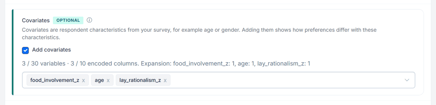
Figure 2. Three covariates selected for the Pizza oven CBC. The line above the chips counts variables and encoded columns.
Tick Add covariates, then open the picker (Select covariates...) and tick variables; Filter variables... searches the list. Each variable shows its type (Nominal, Ordinal, Metric).
The line "3 / 30 variables · 3 / 10 encoded columns" counts what you picked. A metric variable needs one column; a nominal variable needs one column per category minus one.
Choose variables you have a reason to expect an effect from. In the Pizza study these are food_involvement_z and lay_rationalism_z (z-standardized scale scores of the two Likert grids) and age: food involvement should raise the value of a hot oven and the recipe book, lay rationalism the weight of price, and age the preference between dial and touch screen.
Prefer scale scores over single grid items, and avoid variables that measure the same thing twice (income and education, for example); they share the effect and make each one harder to read.
Covariates are available for CBC, CBC Shop, DR-CBC, BW-CBC, MaxDiff and Anchored MaxDiff. In-app covariates are switched on by the platform administrator; when they are off, the panel says "Covariate estimation is currently available in Create Package mode only", when they are on it reads "In-app runs allow up to N encoded covariate columns". The results are explained in sections 4.6 and 4.7.
Curved effects (Spline-HB-L)
By default a numeric covariate acts along a straight line: each additional year of age shifts a part-worth by the same amount. That misses effects that reverse direction, such as a level that the youngest and the oldest respondents both like and the middle age groups do not. The switch Spline-HB-L: Curved effects for numeric covariates lets each numeric covariate follow a curve instead. It sits in the Covariates panel, below the covariate picker.
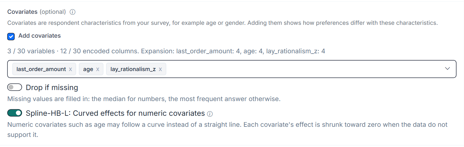
Figure 3. Spline-HB-L switched on: each of the three numeric covariates now uses 4 encoded columns.
Columns. A numeric covariate uses 4 encoded columns instead of 1: 1 for the straight line and 3 for the curve. Variables with very few distinct values can use fewer. The line above the chips shows the count, so check it against the column cap. Nominal variables keep their columns and stay categories.
Shrinkage. Each covariate's effect is shrunk toward zero when the data do not support it. Turning the switch on does not force a bend: without support the curve stays close to a straight or flat line. With few respondents a real bend can also come out flatter than it is.
Availability. The switch exists for in-app runs of CBC, CBC Shop, DR-CBC, BW-CBC, MaxDiff and Anchored MaxDiff. It is hidden under Create Package, and packages estimate straight-line effects.
Switched off, the run is the ordinary straight-line covariate model.
The example in section 4.7 uses three covariates chosen in advance for three expected patterns: age for a U-shaped effect on the controls, lay_rationalism_z for a nearly straight effect on price, and last_order_amount, the amount of the respondent's last pizza order, as a variable with no expected link to the controls of an oven. Both runs used 30,000 + 30,000 iterations and 2 chains and took about 7 to 8 minutes each.
3.5 Variable Coding
For CBC, CBC Shop, DR-CBC and BW-CBC you choose the coding of each attribute in Variable Coding. The form starts with the type set in the variable configuration of the project, otherwise Categorical.
Coding
What It Does
When to Use
Categorical
Effects coding: L−1 columns per attribute (L = number of levels). Produces one part-worth per level.
Brand, colour, feature presence: levels without a natural order, or when you want full flexibility.
Linear
One coefficient per attribute: utility changes by the same amount per unit. Choosing Linear opens a number field per level, pre-filled from numbers in the level labels; check these values.
Price, temperature, warranty length: numeric attributes where you expect a steady effect.
Sign Constraints (Linear attributes only)
As soon as one attribute uses Linear coding, a Sign Constraints block appears with one dropdown per linear attribute ("Forces coefficient signs for linear attributes. Leave blank to let the data decide. Example: price is usually negative (<= 0)."):
No sign constraint (pre-selected): the coefficient may be positive or negative.
Positive (>= 0): for attributes where more should always be better, such as warranty length.
Negative (<= 0): for price-like attributes where more should always be worse.
When to constrain signs
Only constrain with a strong theoretical reason. An unconstrained price coefficient that turns out positive for some respondents may reveal a quality signal; a constraint would hide it. Start unconstrained and constrain only if individual estimates show implausible signs.
3.6 Task-Type Specific Options
Include None Option (DR-CBC and BW-CBC)
DR-CBC always shows Include None Option; BW-CBC shows it when the design fields a None. The follow-up question ("would you buy it?") then enters estimation as a no-choice option with its own constant ASCnone: if a respondent picks a product but answers "No", the task counts as None. A negative ASCnone means respondents generally prefer buying one of the products; a positive one means they often decline. Switch it off to estimate only among the shown products. Traditional CBC and CBC Shop follow the fielded design without a switch.
Choice Contributions (BW-CBC only)
Best + Worst (recommended) uses both answers of each task. Best only and Worst only use one stage, for diagnostic comparisons.
Estimate Display Position Effects (CBC Shop only)
Shop tasks show products in a rendered order, which can influence choice by itself. This checkbox adds control terms for the display positions, so that position effects are separated from the product utilities.
3.7 Advanced MCMC Settings
Click Advanced MCMC Settings at the bottom of the form to open three groups of settings:
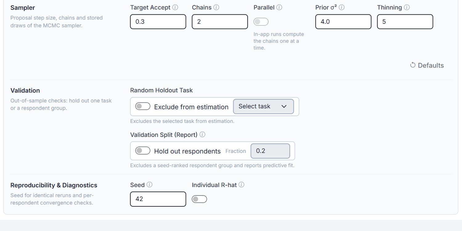
Figure 4. Advanced MCMC Settings of a CBC task.
Group
Setting
What it does
Default
Sampler
Target Accept
Target acceptance rate of the Metropolis-Hastings step (0.1 to 0.5). Around 0.30 works well for most conjoint models (Gelman et al., 2013).
0.3
Chains
Independent chains. At least 2 are needed for R-hat. In-App up to 2, Create Package up to 20.
2
Parallel
Runs the chains at the same time with Julia threads. Only for Create Package; in-app runs compute the chains one at a time, so the switch is disabled there.
Off
Prior σ²
Target prior variance of the respondent covariance matrix. Higher values allow more differences between respondents and less shrinkage.
4.0
Thinning
Keeps every kth draw in the stored histories (1 to 50). Saves memory; it does not improve mixing or ESS.
5
Defaults
Resets Burn-in, Draws, Chains, Prior σ², Thinning, Seed and Target Accept, switches covariates and the respondent holdout off, restores the None option and sets every attribute back to Categorical. Parallel, Individual R-hat and a selected holdout task stay as they are.
Validation
Random Holdout Task
Shown when the design has random tasks. Exclude from estimation plus a task ("Task N") keeps that task out of estimation and scores how well the model predicts it.
Off
Validation Split (Report)
Hold out respondents with a Fraction (0.05 to 0.5) keeps a seed-ranked share of respondents out of estimation and predicts them from the population model (or the covariate model). The utilities of that run then cover the training respondents only.
Off, 0.2
Reproducibility & Diagnostics
Seed
Same seed, data and settings give the same results. An empty field means "Random"; 0 draws a fresh seed. The seed actually used is stored as resolved_seed in Diagnostics.csv.
42
Individual R-hat
Adds a convergence check per respondent (Rhat_Max, Rhat_Mean next to RLH in the individual utilities). Needs at least 2 chains.
Off
MaxDiff and BW-CBC forms differ
BW-CBC and MaxDiff show the validation options as single check rows (Use Random Holdout Task (exclude from estimation), Use Validation Split (Report)). The MaxDiff and Anchored MaxDiff form has no Target Accept and no Thinning (fixed at 0.3 and 5) but an extra field Variance Adj. (default 4.0, 1 to 10), which sets the prior scale of the covariance matrix; its Prior σ² is the prior variance of the population mean (default 1.0, 0.1 to 5.0). The Defaults buttons of these forms also reset Parallel, the None option, Choice Contributions or the holdout task.
3.8 Running the Estimation
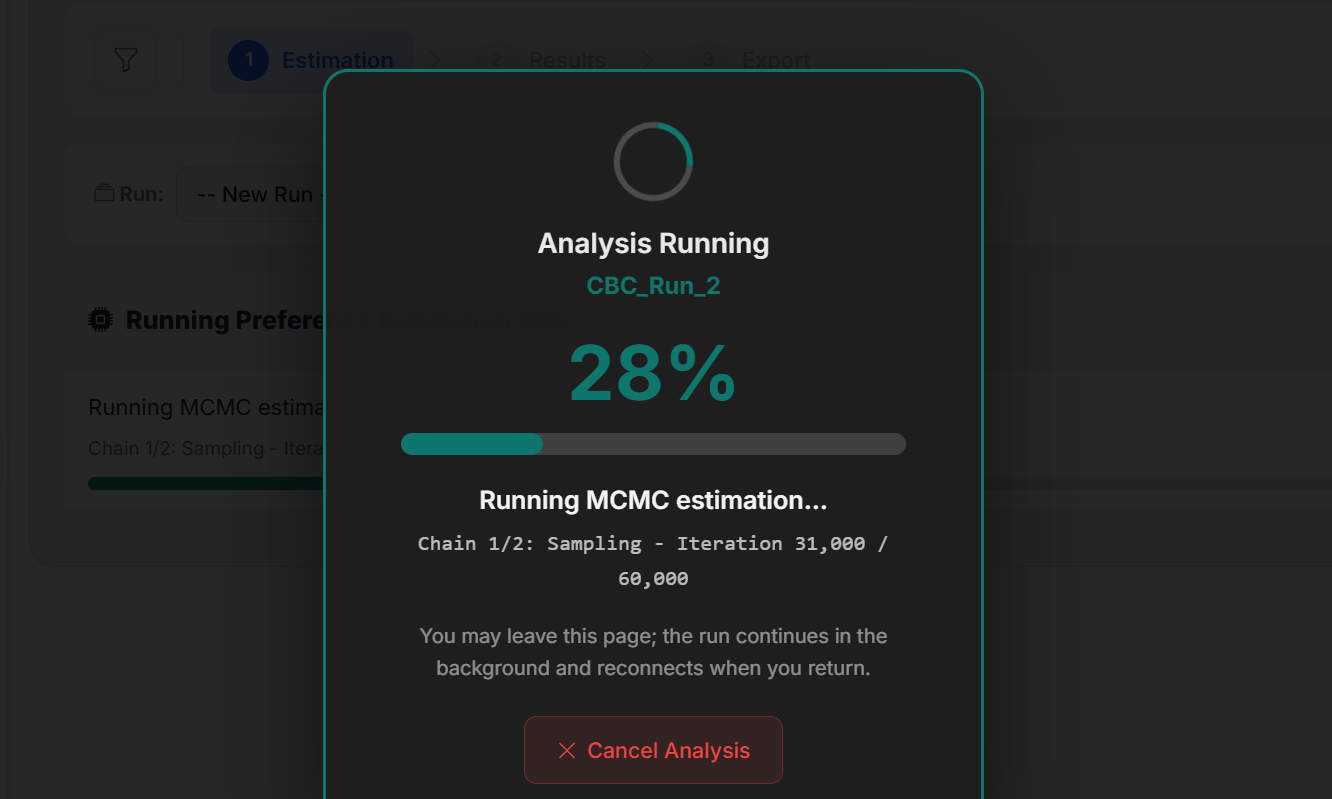
Click Run. A full-screen panel Analysis Running shows the run name, the percentage, the current step ("Running MCMC estimation...") and the iteration of the current chain. Burn-in and draws are counted together, so with 30,000 + 30,000 the counter runs to 60,000 per chain.
Figure 5. A run in progress. You may leave the page; the run continues and the page reconnects when you return.
Cancel Analysis stops the run; partial results are discarded.
At most 3 analyses run at the same time platform-wide. If the server is busy, the dialog "Server Busy" says "The server is currently running X out of Y analyses." and offers Join Queue. The Waiting in Queue card then shows your position and an estimated wait (about 10 minutes per analysis ahead of you), checks every 3 seconds and has a Leave Queue button.
When the run finishes, "Preference Analysis completed!" appears and the page switches to Results.
Typical run times
The Pizza oven CBC (690 respondents, 5 attributes, 3 covariates, 2 chains) took about 2 minutes with 5,000 + 5,000 and about 8 minutes with 30,000 + 30,000. Larger designs take proportionally longer; for very large jobs use Create Package.
4. Interpreting Results
Step 2 of the strip, Results, shows the selected run from top to bottom: the summary bar, attribute importance, average utilities, holdout validation, model diagnostics and, with covariates, the covariate effects and covariate curves. The header has a Download PDF button for the page (the PDF leaves out the covariate curves); most sections have their own PNG button.
4.1 Summary Bar
Figure 6. The summary bar of the Pizza run.
N =: respondents in the run. With a respondent holdout it reads train / total, and a note "Respondent holdout is active." appears below.
Tasks: choice tasks used; Tasks Used:used / total when tasks were excluded.
Active Run: the run shown.
R-hat (max) and ESS (min): the headline convergence figures (section 4.5). Check them first.
Fitted RLH (Posterior Draw Average): average root likelihood of the respondents' own choices (section 12.5). Respondent-Holdout RLH (Posterior-Predictive) is added when the validation split was used.
Acceptance Rate: share of accepted proposals across all iterations, in percent.
Above the bar, the collapsible Estimation details list the observation counts, the run time and, for linear attributes, how the values were centred and scaled.
4.2 Attribute Importance
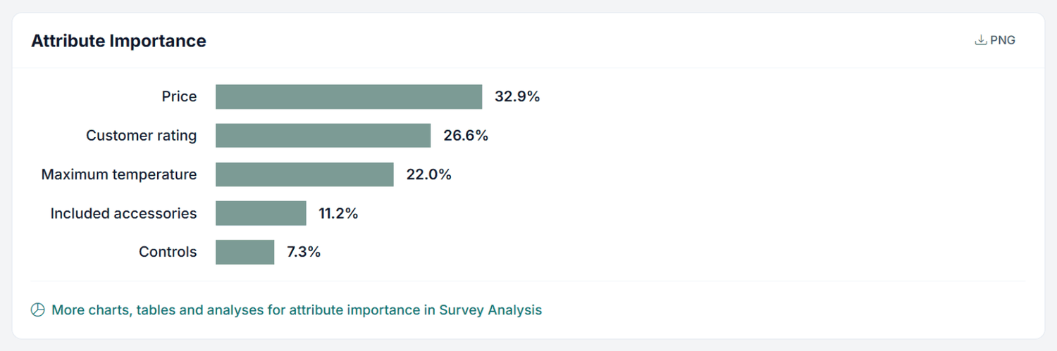
A horizontal bar chart shows each attribute’s relative importance, sorted with the most important attribute at the top. All bars use the same muted teal; the ranking carries the information. A link leads to Survey Analysis for more importance charts and tables.
Importance depends on the level ranges in your design: a price range from $69 to $279 makes price more important than a range from $139 to $209 would.
4.3 Average Utilities
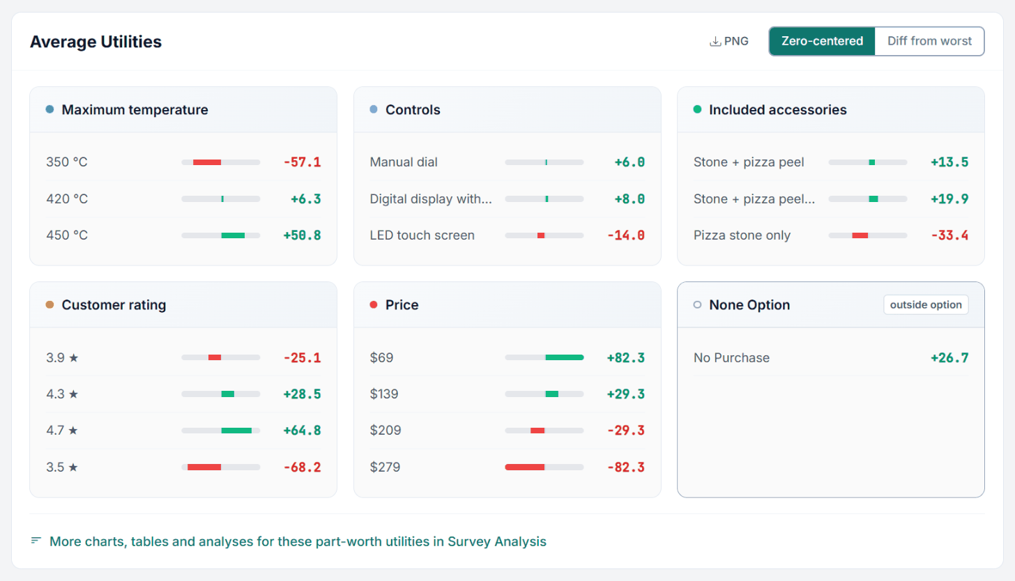
One card per attribute shows the average utility of each level. All cards share one bar scale, so bar lengths can be compared across attributes. A switch in the section header changes the display:
Figure 8. Average utilities (zero-centered) of the pizza oven.
Zero-centered (default): the levels of each attribute sum to zero. Green bars are above the attribute average, red bars below.
Diff from worst: the worst level is set to zero and the others show the gain over it ("switching from 350 °C to 450 °C adds X points").
Linear attributes carry a linear badge and show the slope ("per unit increase", or "across the design range" in Diff from worst) with a footer listing the raw coefficient, the design range and the span.
None option (any run with a None, e.g. DR-CBC): a separate card None Option marked "outside option" with the row No Purchase; it stays zero-centered in both modes ("A single constant has no worst level to count from.").
Interpreting utility values
Utilities are on an interval scale: only differences between levels are meaningful. A utility of +40 for 450 °C does not mean "40 times better"; it means 450 °C is 40 points above the average temperature level. Compare levels within an attribute, and use importances to compare attributes.
4.4 Holdout Validation
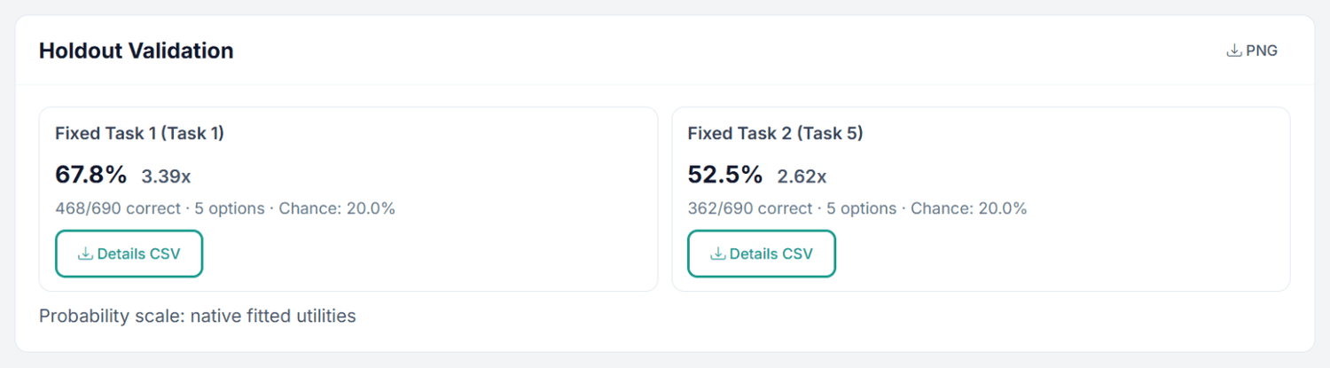
This section appears when the run has tasks that were not used for estimation (the fixed tasks of the design and a random holdout task) or a respondent validation split. One card per task shows:
Figure 9. Holdout Validation for the two fixed tasks of the pizza oven CBC.
Hit rate: share of that task's choices the model predicted correctly (the alternative with the highest predicted utility matches the actual choice).
Ratio: hit rate divided by chance. The pizza oven tasks show four ovens plus None, so chance is 20%: 67.8% correct gives 3.39x.
The line "x/y correct · N options · Chance: z%" and a Details CSV button with the per-respondent predictions.
With a validation split, a Validation Split (Report) card with a Details button appears, and the task cards move under Holdout Task Breakdown. BW-CBC runs get three cards per task: Best, Worst and the exact best-worst pair.
Example: Evaluating Holdout Performance
4-alternative CBC task:
Chance level = 1/4 = 25.0%
Model hit rate = 72.0%
Ratio = 72.0 / 25.0 = 2.88x above chance
Good hit rates for 4-alternative tasks are 60 to 80%; below 50% suggests model problems or very noisy data.
4.5 Model Diagnostics & Fit Metrics
Below Holdout Validation sits the collapsible section Model Diagnostics & Fit Metrics, with CSV and PNG buttons. Click the header to open it. It appears when the run produced at least one of these metrics:
Figure 10. Model Diagnostics & Fit Metrics of the Pizza run.
Metric
Target
What It Measures
If Out of Range
R-hat (max) (summary bar)
< 1.10
Worst between-chain vs within-chain variance ratio across the population-level parameters. Values near 1.0 mean the chains agree.
Use at least two chains, look at the acceptance rate and ESS, and give the run more iterations within the 100,000 budget (or use Create Package).
R-hat (mean)
near 1.0
Average R-hat across the population-level parameters.
Read together with R-hat (max).
ESS (min)
> 400
Effective number of independent draws of the worst parameter. Below 100 is weak.
More post-burn-in draws. Thinning does not help.
Cohen’s Kappa
higher is better
Holdout prediction agreement corrected for chance agreement; the label names the band (Poor, Slight, Fair, Moderate, Substantial, Almost Perfect).
Check design quality and respondent consistency.
MAE / RMSE per alternative / MedAE
lower is better
Error between predicted choice probabilities and observed holdout choices.
Compare across runs.
Multiclass Brier
lower is better
Mean squared error of the predicted probability vector on holdout tasks.
Compare across runs.
Val RLH / Respondent-Holdout RLH (Posterior-Predictive)
well above chance
Root likelihood on held-out data.
Near 1/J the model does not generalize.
Effective Draws
informational
Retained posterior draws behind the diagnostics.
More draws or less thinning if very low.
With a single chain no R-hat can be computed; the R-hat entries are then left out.
When R-hat is above 1.1
Do not report the run. The first Pizza run (5,000 + 5,000 with three covariates) had R-hat (max) 1.33 and ESS (min) 5: its covariance and covariate parameters had not settled. The second run (Figures 6 and 10, 30,000 + 30,000) has R-hat (max) 1.097, just below 1.1, and R-hat (mean) 1.014, but ESS (min) is only 33. The averages are usable for a first look; for a final report run it with more draws in Create Package. More burn-in alone is no automatic cure: give the sampler more iterations overall, keep two chains, and check the acceptance rate.
4.6 Covariate Effects
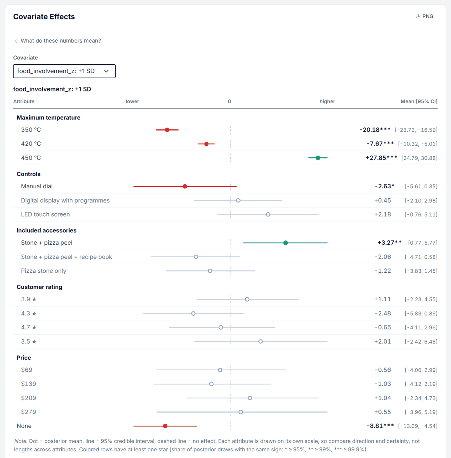
When the run has covariates, the section Covariate Effects appears. At the top, "What do these numbers mean?" explains the figures. Choose a covariate in the Covariate dropdown; the chart shows how one standard deviation more of that covariate (+1 SD) shifts the utility of each level, with 90% credible intervals. The table Effects on Utilities lists the same effects (APA style) with CSV and DOCX buttons; the section's PNG button exports the chart.
Figure 11. Covariate Effects of food_involvement_z in the Pizza run.
In the Pizza run, one standard deviation more food involvement raises the utility of 450 °C by 27.9 points and lowers 350 °C by 20.2 points (*** = at least 99.9% of the posterior draws have the same sign). Rows without a star are drawn grey: there the data give no clear direction.
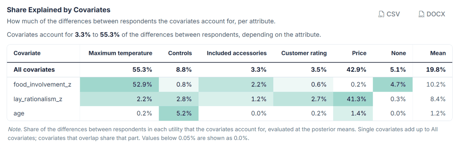
Below follow Effect on Attribute Importances (how a covariate changes the importance of each attribute, computed in ZC-diff space) and Share Explained by Covariates, each with their own CSV and DOCX buttons.
Figure 12. Share Explained by Covariates in the Pizza run: lay rationalism accounts for 41.3% of the differences in price utilities, food involvement for 52.9% of those in maximum temperature, age for 5.2% of those in controls.
The table Share Explained by Covariates shows how much of the differences between respondents the covariates account for. The first row, All covariates, gives this share per attribute; each row below belongs to one covariate and shows its part, sorted by the mean across attributes. The eight largest are visible; Show all N covariates opens the rest. A small share does not make the covariates useless: most differences between respondents come from their own choices, and the covariates mainly describe who prefers what. Covariates that overlap share the part they explain, so a single one can show a very small or slightly negative share while All covariates stays exact; values below 0.05% show as 0.0%.
The table evaluates the shares at the posterior means. The Cov Explained sheet of the Excel export and Covariate_Explained_Share_Summary.csv add a draw-based value averaged over up to 4,000 posterior draws with a 95% interval (NDraws gives the count). It is usually higher, because the uncertainty of the covariate coefficients counts as spread there. The measure is the Bayesian R-squared of Gelman, Goodrich, Gabry and Vehtari (2019), applied to the covariate layer. For attributes with a sign constraint, marked †, the share refers to the log scale used in estimation.
More charts and tables in Survey Analysis
The HB page shows the averages and the covariate model. For the distribution across respondents and for group comparisons, follow the links under Attribute Importance and Average Utilities ("More charts, tables and analyses ... in Survey Analysis"), or open Analysis → Survey Analysis and choose Importances or Part-Worth Utilities under Preference Utilities (HB) in the sidebar.
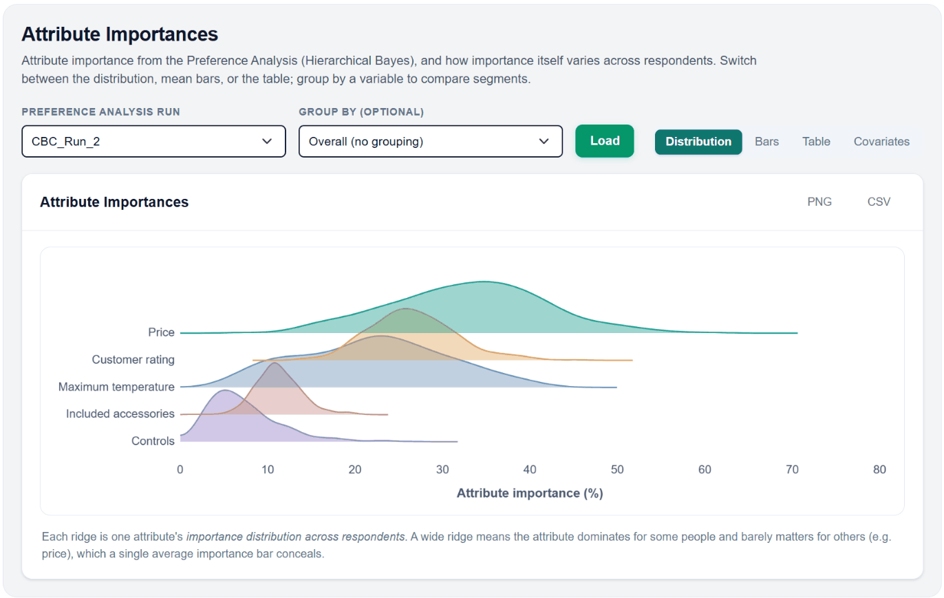
Figure 13. Survey Analysis, Importances: the spread of each attribute's importance across the 690 respondents.
Preference Analysis Run picks the run, Group by (optional) a survey variable for segment comparisons (e.g. gender or diet); Load draws the view.
Distribution shows one ridge per attribute: a wide ridge, like price here, means the attribute dominates for some respondents and barely matters for others. Bars shows the means (per group), Table the numbers, Covariates the relation to the covariates. Every view has PNG and CSV buttons.
Part-Worth Utilities offers the same for the level utilities. The other Survey Analysis pages (Compare Groups, Crosstabs, Correlations, Regressions) work with the respondent characteristics directly.
The HB page shows the effects of the covariates you estimated. To look at the respondent characteristics themselves, or to compare utilities and importances between groups (for example age groups or high vs low food involvement) with charts, crosstabs and tests, open Analysis → Survey Analysis. It reads the individual utilities and importances of your HB runs, so you can use them like any other survey variable. The links under Attribute Importance and Average Utilities lead there directly.
MaxDiff runs show covariate effects with a Percentage points / Utility scale switch and a button "Show N effects with evidence below 95%".
4.7 Covariate Curves
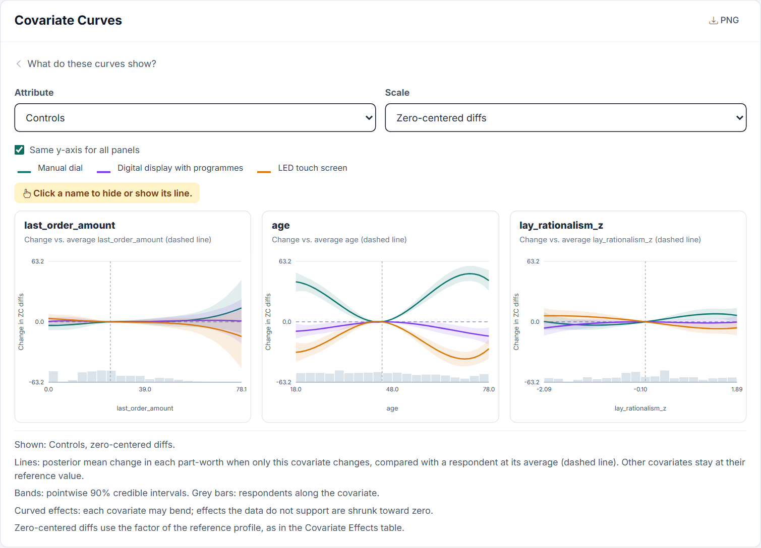
Runs with numeric covariates also show the section Covariate Curves, directly below Covariate Effects. Each panel follows one numeric covariate across the range observed in the sample. The lines show how the part-worths of the selected attribute change when only this covariate changes, compared with a respondent at the covariate's average (dashed line). All other covariates stay at their reference value.
Figure 14. Run with Spline-HB-L, attribute Controls: a U-shaped and an inverted U-shaped effect of age, no clear effect of the last order amount.
The controls of the section
Attribute picks the attribute, the None option, or Attribute importance. There each line is one attribute's importance, in percentage points. Importance is a share of all attributes, so these lines can bend even with straight-line effects.
Scale offers raw utilities, zero-centered diffs (as in the Covariate Effects table) and percent of the attribute's average part-worth range. The percent scale is available for categorical attributes.
Same y-axis for all panels makes the panels comparable. Without it each panel has its own axis, and a tiny effect can look large. The figures in this section use it.
A click on a name in the legend hides or shows its line. The PNG button exports the section, and the Cov Curves sheet of the Excel export holds the numbers.
How to read a panel
Line: the posterior mean change. Above zero means a higher part-worth than a respondent at the average, below zero a lower one.
Band: the pointwise 90% credible interval of that change. Where the band does not contain zero, the data give a clear difference from the average respondent at that value.
Grey bars: how many respondents have that value. Few respondents mean a wide band, so read the ends of a curve with care.
Why the band closes at the dashed line
The change is computed draw by draw against a respondent at the average. At the average itself it is exactly zero in every draw, so no band remains there, and the band widens with the distance from the average. This does not mean the utility of an average respondent is known exactly: the band answers how sure the difference from the average respondent is. The uncertainty of the utility level itself is not part of it.
Three patterns in the Pizza run
U shape. In Figure 14, the manual dial is worth about 42 points more at age 18 and about 43 points more at age 78 than at the average age of 45. The LED touch screen mirrors this as an inverted U, about 32 points lower at age 18 and 28 points lower at age 78. Young and old respondents thus differ from the middle age groups in the same direction.
No effect. In the left panel of Figure 14, the bands of all three controls contain zero along the entire range of last_order_amount. The lines fan out at the right end, where few respondents spent that much, and the band widens with them. In the table Share Explained by Covariates, this covariate accounts for 0.2% of the differences in the controls. No effect on one attribute says nothing about the others: the same covariate does shift the utility of the None option.
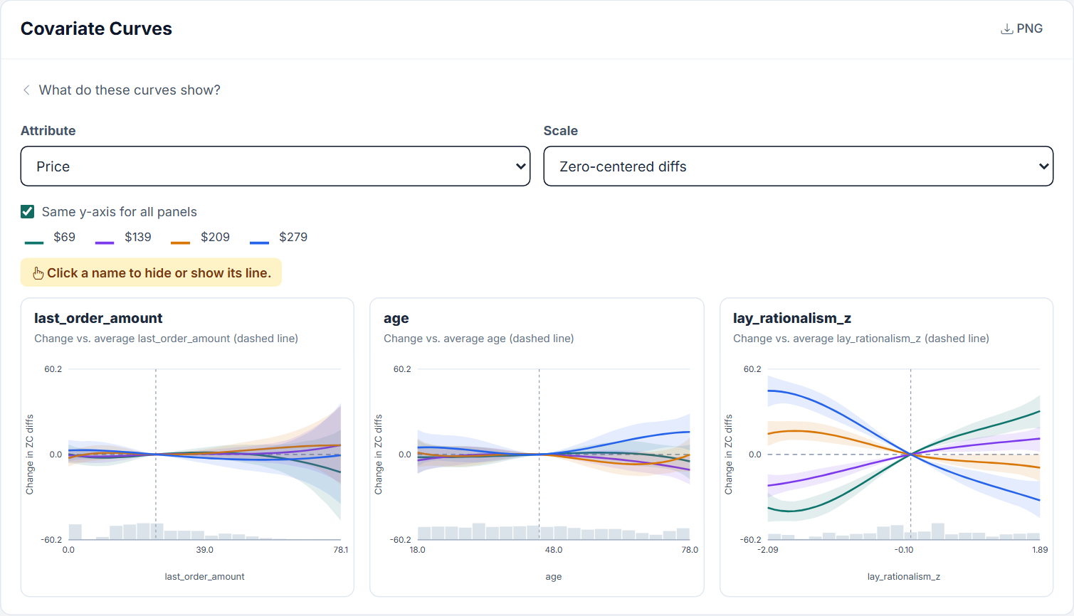
Figure 15. Run with Spline-HB-L, attribute Price: a nearly straight effect of lay rationalism.
Nearly straight. In the right panel of Figure 15, the higher the lay rationalism, the more the low prices gain and the high prices lose. From the lowest to the highest value, $69 moves from about −38 to +31 points and $279 from about +45 to −32 points. The lines flatten a little at the ends, but a straight line would describe them well. Spline-HB-L leaves such an effect close to a straight line.
Straight line versus curve
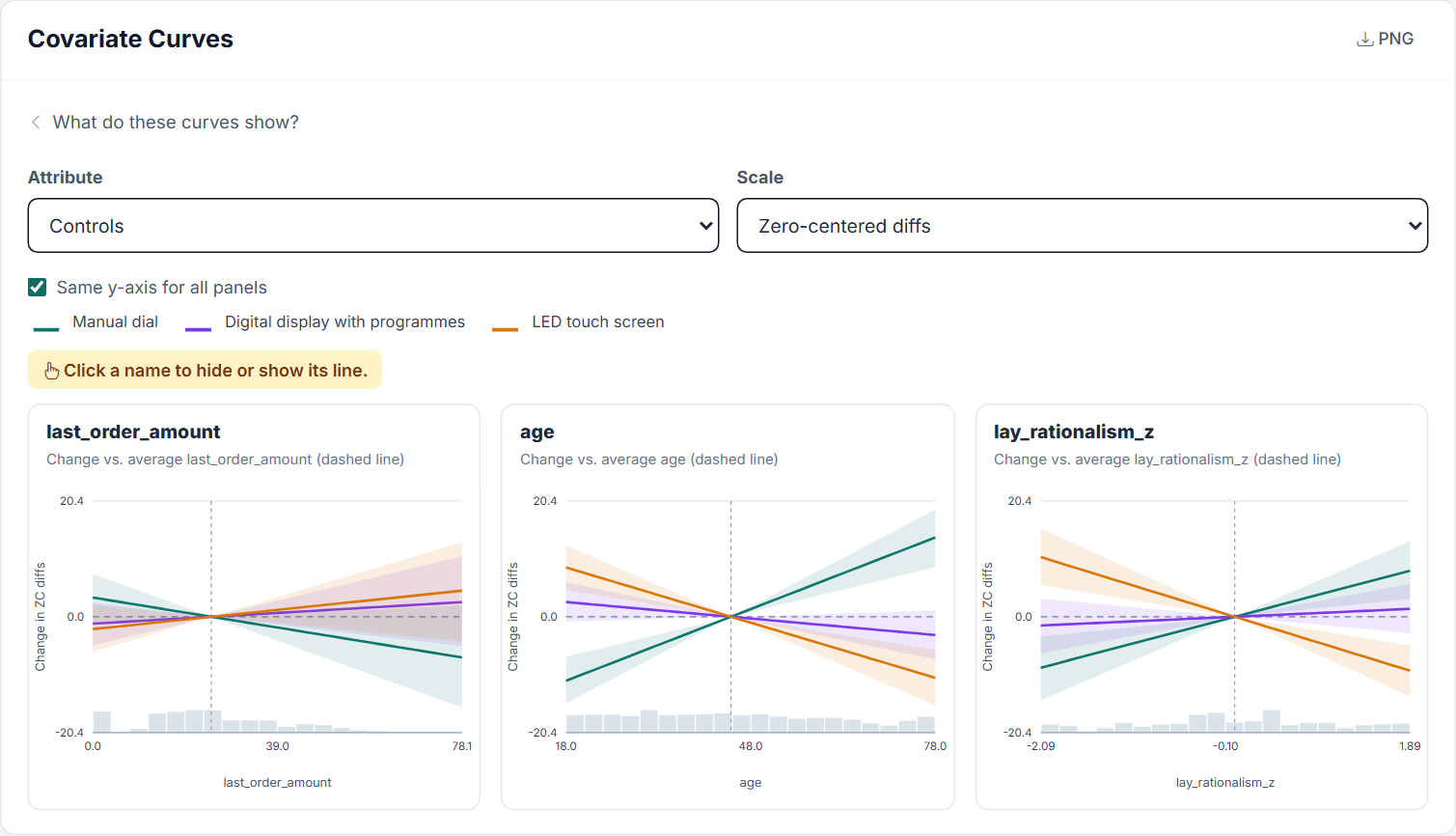
Figure 16. The same covariates and attribute without Spline-HB-L. All lines are straight. Note the smaller y-axis.
The straight-line run in Figure 16 reports a steady rise of the manual dial with age, from about −11 points at age 18 to about +14 points at age 78. For the older half that points in the right direction but is far too small; for the younger half it points in the wrong direction. The covariates' share of the differences in the controls shows the same gap: age accounts for 31.8% with curves and 5.2% with straight lines.
The prediction of the choices themselves changed little in this example: Fitted RLH 0.633 with curves and 0.629 without, hit rate on the fixed tasks 58.8% and 58.5%. The curves mainly improve the description of who prefers what.
What to keep in mind
The Covariate Effects table shows the straight part only. In a run with Spline-HB-L, the "+1 SD" columns and the chart in section 4.6 hold the linear coefficient, not the curve. Here the table gives age only +4.65 on the manual dial, while the curve reaches about +38 points at age 63. For a curved effect, read the curves; a small "+1 SD" effect does not mean there is no effect. Share Explained by Covariates counts the straight part and the curve together.
Check convergence first. The curve parameters are part of R-hat and ESS. This run reached R-hat (max) 1.07 but only ESS (min) 35, below the guideline of 400, so it serves as an illustration; for a final report run more iterations.
Choose covariates with a reason. A curve found by trying many covariates can be chance. A curve describes a relation in your sample, not a cause.
Runs without the switch show this section as well, with straight lines. Sign-constrained linear attributes are estimated on a log scale, so their lines can bend even then.
MaxDiff and Anchored MaxDiff show one panel per covariate for the selected Item, in Relative Preference percentage points or on the utility scale. The anchor threshold of Anchored MaxDiff has its own entry, on the utility scale only.
5. Exporting Results
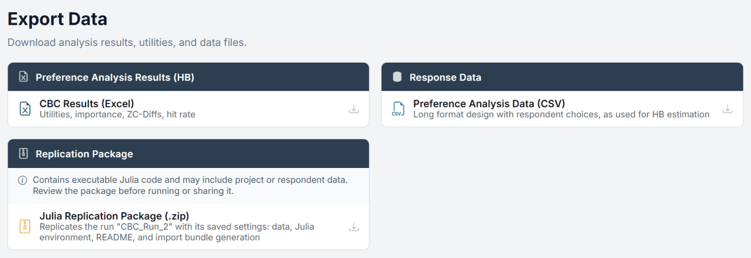
Step 3 of the strip, Export, opens Export Data once a run has results. It groups the files into three cards:
Figure 17. The Export step of the Pizza run.
Card
Download
Contents
Preference Analysis Results (HB)
CBC Results (Excel) (MaxDiff Results (Excel) on MaxDiff tasks)
The workbook described below.
Preference Analysis Results (HB)
Parameter Diagnostics (CSV) (DR-CBC)
R-hat and ESS for each estimated parameter. For the other types they are in the workbook sheet Parameter_Diagnostics.
Response Data
Preference Analysis Data (CSV) (on MaxDiff: MaxDiff Responses (Long Format), a ZIP with data.csv and attributes.csv)
The long-format data used as input for estimation.
Replication Package
Julia Replication Package (.zip)
With a selected run: replicates that run with its saved settings and exactly its participants. Without a run: the same package Create Package produces from the current form.
The Excel workbook contains, in this order: Summary, Settings & Diagnostics (design, HB settings actually used, RLH statistics with chance RLH, flagged respondents, holdout figures, Bulk and Tail ESS), Individual_ZC_Diffs, Individual_Raw, Individual_Importances, with linear attributes Linear_Coefficients_Raw and Linear_Coefficients_ZC, Flagged_Respondents, with covariates Cov Effects (Raw), Cov Effects (ZC), Cov Importances and Cov Explained, with a validation split Validation Split (Report), and finally Parameter_Diagnostics and Estimation Audit.
Reproducibility best practice
Download the Julia Replication Package for final or published analyses, right after the run finishes. It takes the run's participant list, but the answers are read from the project at download time: participants deleted later are missing, and answers edited later appear in their edited form. The README states which run it replicates and how many of its participants it contains. The package contains executable code and may contain respondent data; review it before running or sharing it.
6. What to Do After HB
HB estimation is the starting point. The individual utilities feed these analyses:
Market Simulation: header menu Analysis → Market Simulation (MaxDiff Simulation for MaxDiff tasks). Simulates shares of preference, price curves and competitive scenarios from a run with results.
Willingness to pay: in the Market Simulation, converts utility differences into money. It works with linear and categorical price coding.
Survey Analysis: header menu Analysis → Survey Analysis. Compares utilities and importances between respondent groups with charts, crosstabs and tests.
AI-Driven Profile Analysis (second tab): TasteNet-MNL, for preference weights that change with respondent characteristics, not only shift with them.
Latent Class (third tab): discovers segments with distinct preference profiles.
Interaction Effects (fourth tab): tests which attribute interactions matter.
Workflow recommendation
(1) Run HB, (2) check R-hat, ESS and the holdout fit, (3) look at importances and utilities, (4) add covariates you have reasons for and compare groups in Survey Analysis, (5) run simulations for the business questions, (6) run Latent Class for segmentation.
7. Best Practices & Common Pitfalls
Do
Check R-hat (max) < 1.1 and ESS (min) > 400 before trusting results. Raise the iterations when they are out of range, especially with covariates.
Use 2 chains, so that R-hat can be computed.
Keep the fixed holdout tasks of the design and look at their hit rates.
Report Fitted RLH together with the chance RLH.
Choose covariates with a reason, prefer scale scores, and avoid overlapping variables.
Switch on Spline-HB-L when a numeric covariate may not act along a straight line, and read those effects in the Covariate Curves, not in the "+1 SD" table.
Compare several runs with different settings to check that the results are robust.
Don’t
Don’t report a run with R-hat > 1.1.
Don’t compare raw utility magnitudes across respondents. Use importances or ZC-Diffs; utility scales differ between respondents.
Don’t use HB utilities as segments. HB assumes one continuous population distribution; use Latent Class for discrete segments.
Don’t expect interaction terms: HB estimates main effects. Use Interaction Effects to test whether interactions matter.
Don’t run HB with fewer than 30 respondents.
The “more is always better” trap
More draws give more precise averages, with diminishing returns once R-hat and ESS are fine. If results change substantially between two converged runs, look for a convergence or design problem rather than adding draws.
Part II
Theoretical Background
The statistical foundations of HB estimation, for methodologists, reviewers, and the deeply curious.
8. Key Definitions
Glossary
Hierarchical Bayes (HB)
A two-level Bayesian model that borrows strength across respondents. Level 1 models individual choices; Level 2 models the population distribution of preferences.
Spline-HB-L
The HB model with covariates in which numeric covariates keep a straight-line column and gain a curve block that is shrunk toward zero when the data do not support it (sections 3.4, 4.7 and 9.2).
MCMC (Markov Chain Monte Carlo)
A simulation-based method for sampling from posterior distributions that are analytically intractable. The chain is “Markov” because each draw depends only on the previous draw, and “Monte Carlo” because it uses random simulation.
Gibbs Sampling
An MCMC method that draws each parameter from its conditional posterior distribution (given all other parameters). Used in HB for population-level parameters (μ and Σ) where closed-form conditionals exist.
Metropolis-Hastings (MH)
An MCMC method that proposes new parameter values from a proposal distribution and accepts or rejects based on the likelihood ratio. Used in HB for individual-level betas where no closed-form conditional exists.
Burn-in
Initial MCMC iterations discarded before the chain reaches its stationary distribution. The chain needs time to “forget” its arbitrary starting values.
Part-Worth Utilities
Preference weights estimated for each attribute level. Higher utility = more preferred. Only differences between levels are meaningful (interval scale).
Zero-Centered Diffs (ZC-Diffs)
Rescaled utilities where each attribute’s levels sum to zero, and the average attribute range is normalized to 100. This standardization enables comparison across attributes and studies.
Root Likelihood (RLH)
The geometric mean of the predicted probability of the chosen alternative across all choice tasks. RLH = 1.0 is perfect prediction; RLH = 1/J (where J = number of alternatives) is chance level.
R-hat (Gelman-Rubin Diagnostic)
A convergence diagnostic comparing between-chain variance to within-chain variance. Values near 1.0 indicate convergence; values above 1.1 indicate the chains have not mixed.
Effective Sample Size (ESS)
The number of effectively independent MCMC draws after accounting for autocorrelation. A chain of 10,000 draws with high autocorrelation might have ESS of only 500.
Shrinkage
The tendency of HB to pull individual estimates toward the population mean. Respondents with noisy data are shrunk more; respondents with clear patterns are shrunk less. This is statistically optimal (James-Stein estimation).
9. The Two-Level Hierarchical Model
9.1 Level 1: Individual Choice Model (MNL)
At the individual level, each respondent i is modeled by a Multinomial Logit (MNL) model with their own preference vector βi:
Vij = Xj · βi
Deterministic utility of alternative j for respondent i
P(j chosen | βi) = exp(Vij) / ∑k exp(Vik)
Multinomial Logit choice probability (softmax)
Here Xj is the design vector describing alternative j (coded attribute levels), and βi is respondent i’s vector of part-worth utilities. The probability of choosing alternative j increases with its utility relative to all other alternatives in the choice set.
9.2 Level 2: Population Distribution
The second level specifies how individual preference vectors are distributed across the population:
βi ~ MVN(μ, Σ)
Individual preferences drawn from a multivariate normal distribution
μ (mu) = the population mean preference vector. This represents the “average respondent.”
Σ (Sigma) = the population covariance matrix. This captures both (a) how much individual preferences vary around the mean and (b) the correlations between preferences for different attributes.
The multivariate normal assumption is powerful because it captures preference correlations. For example, if respondents who prefer Brand A also tend to be less price-sensitive, this correlation appears as an off-diagonal element in Σ.
Covariates and Spline-HB-L
With covariates, the population mean depends on the respondent. Each respondent has a row vector zi of encoded covariate columns with a leading 1, and the coefficient matrix A has one row per column:
βi ~ MVN(A′ zi, Σ)
The first row of A is the intercept; the other rows are the covariate effects
With Spline-HB-L each numeric covariate contributes two parts to zi. The linear column is the standardized covariate; category dummies are standardized in the same way. The curve block is built from a cubic B-spline with three knots at the minimum, median and maximum of the training respondents. Its columns are residualized against the intercept and all linear columns, rotated onto their remaining directions (at most 3 columns) and scaled to unit variance. The block therefore carries only the part of the effect beyond the straight lines.
The intercept keeps its fixed prior. Every linear column is its own group g, and every curve block forms one group. Each group has its own adaptive scale τg, drawn in the Gibbs sampler after Σ:
For every row r of A in group g. A small τg shrinks the whole group toward zero, which is why a curve without support in the data stays flat.
Reports convert the draws exactly, without changing any prediction: linear rows per unit of the usual covariate coding (per SD for numeric covariates, versus the reference for categories), curve columns shifted to zero at the reference profile. Covariate Curves evaluate each draw along the observed range and take the difference from the reference draw by draw.
9.3 Prior Distributions
Being Bayesian, the model requires prior distributions on the population parameters:
μ | Σ ~ MVN(0, σ2mean · Σ)
Conjugate normal prior on the population mean, scaled by the current covariance (σ2mean = 100)
Σ ~ Inverse-Wishart(K + 5, 4 · V)
Prior on the population covariance. V is the target covariance built from Prior σ²: 4.0 on the diagonal for linear and none-option coefficients, and the effects-coded block ((L−1)/L · 4 on the diagonal, −4/L off the diagonal) for a categorical attribute with L levels. With df = K + 5 the prior mean of Σ equals V, which is why the field is called the target prior variance.
This is the prior for CBC, CBC Shop and BW-CBC. DR-CBC uses μ ~ N(0, 100 · I), not scaled by Σ. MaxDiff and Anchored MaxDiff use μ ~ N(0, Prior σ² · I) with the MaxDiff field Prior σ² (default 1.0), and their Inverse-Wishart scale comes from the field Variance Adj.
Choicery uses diffuse (weakly informative) priors by default, centered at zero. The two variances are separate: the prior on the population mean uses a fixed, very diffuse σ2mean = 100.0 that is not exposed in the UI, while the Inverse-Wishart scale on Σ defaults to σ2prior = 4.0 and is editable in Advanced MCMC Settings as Prior σ². These priors have minimal influence on the posterior when you have a reasonable amount of data (> 50 respondents). The Inverse-Wishart prior on Σ ensures positive-definiteness of the estimated covariance matrix.
The Inverse-Wishart degrees of freedom are fixed at dfprior = K + 5, where K is the number of estimated parameters. This is the external benchmark default and the industry convention. The "+5" offset (referred to internally as df_offset) is not exposed in the UI because: (a) at typical sample sizes (n > 200) it has negligible impact on the posterior (the likelihood dominates), and (b) departing from K+5 only makes sense for very specific academic replications. If you need a non-default value (e.g. K+2 for a paper using a more diffuse Σ-prior), edit the offline HB package's hb_analysis.jl directly and re-upload via the import path.
9.4 Shrinkage: The Key Insight
The most important property of HB estimation is shrinkage: individual estimates are pulled toward the population mean. The degree of shrinkage depends on the relative informativeness of the individual’s data vs. the population distribution.
βiHB ≈ wi · βiMLE + (1 − wi) · μ
Shrinkage: HB estimate is a weighted average of individual MLE and population mean
If respondent i has many tasks and clear patterns → high wi → estimate stays close to their individual data.
If respondent i has few tasks or noisy choices → low wi → estimate is pulled toward the population mean.
This is optimal in a mean-squared-error sense (the James-Stein phenomenon). Even when individual estimates are slightly biased toward the mean, the overall accuracy across all respondents is higher than individual-level MLE (Allenby, Arora, & Ginter, 1995).
Shrinkage is a feature, not a bug
New users sometimes worry that HB “distorts” individual estimates. In fact, shrinkage improves them. With only 12 choice tasks per respondent, individual MLE estimates are extremely noisy. By borrowing information from the population, HB produces estimates that are, on average, closer to each respondent’s true preferences (Huber & Train, 2001).
10. The MCMC Sampling Algorithm
The posterior distribution of the HB model is analytically intractable: there is no closed-form solution. Instead, Choicery uses MCMC to draw samples from the posterior, and these samples are used to estimate posterior means, standard deviations, and other quantities of interest.
10.1 Gibbs Sampling with Metropolis-Hastings Steps
Choicery’s HB implementation uses a Gibbs sampler that cycles through three steps in each iteration:
1
Sample individual betas βi (Metropolis-Hastings). For each respondent, propose a new βi from the current value plus a scaled multivariate normal perturbation. Accept or reject the proposal based on the Hastings ratio:
where L(β) is the choice likelihood and p(β | μ, Σ) is the MVN population density.
2
Sample population mean μ (conjugate Gibbs). Given all individual βi and the current Σ, the conditional posterior of μ is a multivariate normal with a closed-form mean and covariance. This is a direct draw: no accept/reject needed.
3
Sample population covariance Σ (conjugate Gibbs). Given all individual βi and the current μ, the conditional posterior of Σ is an Inverse-Wishart distribution. Again, this is a direct draw from a known distribution.
With upper-level covariates, step 2 draws the full coefficient matrix (intercept row = population mean, one row per encoded covariate column) from its matrix-normal conditional instead of μ alone. These three steps are repeated for n_burn + n_draws total iterations. The first n_burn iterations are discarded (burn-in), and the remaining n_draws iterations provide the posterior samples.
10.2 Adaptive Proposal Scaling
The Metropolis-Hastings step requires a proposal distribution. Choicery uses a multivariate normal proposal centered at the current βi, with a scale parameter that controls the “step size.”
Each respondent has an own proposal scale, starting at 0.1. During burn-in it is adaptively tuned every 100 iterations: if the acceptance rate is more than 0.05 above the target (default 0.30) the scale grows by 10%, if it is more than 0.05 below it shrinks by 10%, always between 0.001 and 2.0. After burn-in, the scale is fixed. You steer this only through Target Accept; the scale itself is not a setting.
Why 30% acceptance?
Theoretical results (Roberts & Rosenthal, 2001) show that ~23.4% is optimal for high-dimensional targets. In practice, 25 to 35% works well for conjoint models. Too high (>50%) means the chain moves in tiny steps and explores slowly. Too low (<10%) means most proposals are rejected and the chain gets stuck.
10.3 Multiple Chains
Choicery runs independent chains with different random seeds: 1 or 2 for in-app runs (2 is the default and the in-app maximum), up to 20 in a Create Package run. Every chain starts from the same neutral point (small random betas, μ = 0, Σ = prior) and then follows its own random path. Multiple chains serve two purposes:
Convergence assessment: if chains with different random paths settle on the same distribution, this is strong evidence of convergence (R-hat diagnostic).
More posterior samples: draws from all chains are pooled for final estimates, increasing ESS.
In Create Package runs with Parallel switched on, chains run simultaneously on separate CPU cores, with near-linear speedup. In-app runs compute the chains one after the other.
11. Convergence Diagnostics
MCMC convergence is the single most important quality check for HB results. A non-converged chain produces meaningless results. Choicery reports R-hat (max), ESS (min) and the overall acceptance rate in the summary bar, R-hat (mean) and ESS (min) again in Model Diagnostics & Fit Metrics, and the acceptance of each chain in the run progress.
11.1 R-hat (Gelman-Rubin Diagnostic)
R-hat compares the variance between chains (B) with the variance within each chain (W). If chains have converged to the same distribution, these should be similar.
var_hat = ((n−1)/n) · W + (1/n) · B
R-hat = √(var_hat / W)
Choicery implements the modern rank-normalized split R-hat of Vehtari, Gelman, Simpson, Carpenter and Bürkner (2021): each chain is split in half, draws are rank-normalized, and the larger of the bulk and the folded (scale) statistic is reported. It is computed on the stored upper-level draws, that is the population mean (or the covariate coefficient rows) and the elements of the covariance matrix.
R-hat Value
Interpretation
Action
< 1.05
Excellent convergence
Results are reliable.
1.05 to 1.10
Acceptable convergence
Results are usable. Consider more iterations for critical analyses.
> 1.10
Not converged
Review acceptance rate and ESS, then reallocate burn-in versus post-burn-in draws and re-run with at least two chains. Use Create Package if more than the in-app budget is justified.
Choicery reports the maximum R-hat across these population-level parameters as R-hat (max) in the summary strip (per-respondent convergence is only checked when Individual R-hat is switched on). Even if most parameters have excellent R-hat, a single parameter with R-hat > 1.1 means the model has not fully converged.
11.2 Effective Sample Size (ESS)
MCMC draws are autocorrelated: consecutive draws tend to be similar. ESS tells you how many independent samples your chain is equivalent to:
ESS = n / (1 + 2 · ∑k=1K ρk)
Effective sample size, where ρk is the autocorrelation at lag k
This is the simplified textbook form. Choicery computes the rank-normalized split bulk ESS with Geyer's initial-sequence method, plus a tail ESS (Vehtari et al., 2021); the workbook reports Bulk ESS (min), Bulk ESS (mean) and Tail ESS (min). A chain of 10,000 draws with high autocorrelation might have ESS of only 500. Thinning (keeping every kth draw) reduces stored samples but does not improve ESS per wall-clock time. It mainly saves memory.
Target: ESS > 400 for reliable posterior mean estimates. For posterior quantiles (e.g., 95% credible intervals), ESS > 1,000 is preferred.
11.3 Acceptance Rate
The acceptance rate is the percentage of Metropolis-Hastings proposals that are accepted. It is a proxy for how well the proposal distribution matches the posterior.
Acceptance Rate
Interpretation
< 15%
Proposals are too aggressive. Chain gets stuck at current values. Check whether burn-in was long enough for the adaptation, and the Target Accept setting.
20 to 35%
Optimal range. Chain explores efficiently.
> 50%
Proposals are too conservative. Chain moves in tiny steps and mixes slowly. Check the Target Accept setting and the burn-in length.
12. Post-Processing: From MCMC Draws to Utilities
After MCMC sampling completes, the raw draws must be post-processed into usable utility estimates. Choicery performs these steps automatically:
12.1 Posterior Mean
For each respondent i, the final utility estimate is the average (posterior mean) of all post-burn-in draws:
βiHB = (1/D) · ∑d=1D βi(d)
Posterior mean over D post-burn-in draws
12.2 Reference Level Recovery (Effects Coding)
Effects coding estimates L−1 coefficients for an attribute with L levels. The reference level’s utility is recovered as:
βref = − ∑l=1L-1 βl
Reference level = negative sum of estimated levels
12.3 Zero-Centered Diffs (ZC-Diffs)
To enable cross-attribute comparison, utilities are rescaled so that the average attribute range equals 100:
Recover the reference level (12.2), so the levels of each categorical attribute already sum to zero.
For each attribute, compute the range: max(utility) − min(utility).
Compute the average range across all attributes.
Multiply all utilities, including ASCnone, by 100 / average_range.
This is done per respondent, so every respondent's utilities are on the same scale.
12.4 Attribute Importance
Importancea = rangea / ∑all a rangea × 100%
Relative importance as share of total utility range
Importances are computed at the individual level first, then averaged. This individual-level averaging is more appropriate than computing importances from averaged utilities (Orme, 2020).
12.5 Root Likelihood (RLH)
RLHi = exp( (1/Ti) · ∑t=1Ti log P(yit | βi) )
Geometric mean of predicted probabilities across T tasks
Choicery evaluates this quantity for every 10th post-burn-in draw of βi and averages the results, rather than plugging in the posterior mean. This posterior-draw average is the value shown as Fitted RLH.
RLH is the geometric mean of the predicted probability of each respondent’s chosen alternative. It ranges from 1/J (chance level, where J = number of alternatives) to 1.0 (perfect prediction). A “good” RLH depends on the number of alternatives:
Alternatives (J)
Chance RLH
Good RLH
Excellent RLH
3
0.333
0.55 to 0.70
> 0.70
4
0.250
0.45 to 0.60
> 0.60
5
0.200
0.40 to 0.55
> 0.55
13. Design Matrix and Coding
The design matrix X encodes the attribute levels of each alternative in a format suitable for estimation. Choicery supports three coding schemes:
13.1 Effects Coding (Categorical Attributes)
For an attribute with L levels, effects coding creates L−1 columns. The reference level (last level) is coded as −1 on all columns:
The reference level’s utility is recovered as βC = −(βA + βB). Effects coding ensures that utilities sum to zero across levels, which is required for zero-centered diffs.
13.2 Linear Coding (Numeric Attributes)
A single column contains the centered and rescaled attribute values: Choicery subtracts the mean of the levels and divides by half their range. For evenly spaced levels the sampler then works on values between −1 and +1 (here −1, −0.33, +0.33, +1). Results are converted back, so the reported coefficient is per raw unit and each level’s utility is β times (price minus mean):
The ASCnone coefficient captures the baseline tendency to choose (negative) or avoid (positive) the none option, independent of product attributes.
14. HB vs. Other Estimation Methods
HB is one of several estimation methods for conjoint data. The table below summarizes when to use each approach:
Method
Individual-Level
Heterogeneity
Segmentation
Speed
When to Use
Aggregate MNLside output only
No
Ignored
No
Instant
Not offered as a standalone analysis. HB shares the same multinomial-logit likelihood and recovers the aggregate solution as a special case when heterogeneity vanishes, but it additionally delivers individual-level part-worths, credible intervals, and direct inputs for simulation, WTP, and holdout validation. If you still need aggregate utilities, run the Interaction Effects analysis and open its Excel export: the sheet Main Effects (Aggregate MNL) contains the full main-effects MNL fit. Alternatively, any Latent Class run also estimates the 1-class aggregate (pooled MNL) baseline as a reference solution.
Run HB for individual-level utilities → use for simulation, WTP, and individual-level analysis. Run LC for segmentation → use for segment strategy, targeting, and profiling.
They answer different questions. HB asks “what does this respondent prefer?” LC asks “what types of respondents exist?”
Why Choicery Does Not Offer Aggregate MNL
Aggregate MNL estimates a single set of utilities for the entire sample and ignores preference heterogeneity. When preferences vary across respondents (which they almost always do), the aggregate coefficients are biased and standard errors are understated. Crucially, aggregate MNL cannot produce the individual-level utilities that every downstream Choicery module (Market Simulator, WTP, Price Elasticity, Reservation Price, Hit-Rate, Sensitivity) depends on.
Because HB uses the same multinomial-logit likelihood and degenerates to the aggregate solution in the limit of zero heterogeneity, it strictly dominates aggregate MNL: you get the aggregate picture plus the individual posterior, with no realistic scenario in which aggregate MNL would give a better answer. Offering it as a separate option would invite the biased-estimate trap without adding capability, so Choicery provides HB (and, for discrete segments, Latent Class) as the only supported estimators. For the rare cases where aggregate utilities are genuinely needed (for example as a textbook baseline), two indirect routes exist: the Main Effects (Aggregate MNL) sheet of the Interaction Effects Excel export, and the 1-class baseline solution that every Latent Class run estimates alongside the multi-class models.
Why Not Cluster HB Utilities Instead of Running LC?
You can cluster HB utilities using k-means or hierarchical clustering, but this is suboptimal. LC simultaneously estimates segment membership and segment-specific preferences, which produces more coherent segments than a two-step approach. However, clustering HB utilities can be useful as a quick exploratory tool or when you need more flexibility in the clustering algorithm.
15. References
Allenby, G. M., Arora, N., & Ginter, J. L. (1995). Incorporating prior knowledge into the analysis of conjoint studies. Journal of Marketing Research, 32(2), 152-162.
Gelman, A., Carlin, J. B., Stern, H. S., Dunson, D. B., Vehtari, A., & Rubin, D. B. (2013). Bayesian data analysis (3rd ed.). Boca Raton, FL: CRC Press.
Gelman, A., Goodrich, B., Gabry, J., & Vehtari, A. (2019). R-squared for Bayesian regression models. The American Statistician, 73(3), 307-309.
Huber, J., & Train, K. (2001). On the similarity of classical and Bayesian estimates of individual mean partworths. Marketing Letters, 12(3), 259-269.
Lenk, P. J., DeSarbo, W. S., Green, P. E., & Young, M. R. (1996). Hierarchical Bayes conjoint analysis: Recovery of partworth heterogeneity from reduced experimental designs. Marketing Science, 15(2), 173-191.
Orme, B. K. (2020). Getting started with conjoint analysis (4th ed.). Manhattan Beach, CA: Research Publishers LLC.
Orme, B. K., & Chrzan, K. (2017). Becoming an expert in conjoint analysis. Orem, UT: external conjoint software.
Rao, V. R. (2014). Applied conjoint analysis. Berlin: Springer-Verlag.
Rossi, P. E., Allenby, G. M., & McCulloch, R. (2005). Bayesian statistics and marketing. Chichester: Wiley.
Vehtari, A., Gelman, A., Simpson, D., Carpenter, B., & Bürkner, P.-C. (2021). Rank-normalization, folding, and localization: An improved R-hat for assessing convergence of MCMC (with discussion). Bayesian Analysis, 16(2), 667-718. doi:10.1214/20-BA1221
external conjoint software. (2009). The CBC/HB system for hierarchical Bayes estimation [Technical paper]. Orem, UT: external conjoint software.