
How to measure the monetary value of product features using conjoint analysis, a practical guide for Choicery with methodological background.
How to use WTP analysis in Choicery, step by step, with examples.
Willingness to Pay (WTP) answers a simple question: "How much more would consumers pay for this feature?"
For example, if you run a conjoint study about cars and want to know how much extra people would pay for an SUV compared to a Sedan, WTP gives you a concrete Euro amount.
Choicery offers three WTP methods on the WTP tab of the Market Simulator. Each one has its own sub-tab directly under the tab heading: Simulation WTP, Robust WTP and Pseudo-WTP. Only one sub-tab is shown at a time, and each sub-tab keeps its own result.
| Sub-tab | What It Does | When to Use |
|---|---|---|
| Simulation WTP | Simulates the full competitive market with the products you defined under PRODUCTS. Raises the price of the improved product until its simulated preference share drops back to baseline. The price increase = WTP. | When you have a well-defined, stable competitive landscape with specific competitors. |
| Robust WTP Sampling of Scenarios (SOS) |
Runs the same break-even calculation across hundreds of randomly generated competitive scenarios. Reports the median WTP with bootstrap 95% confidence intervals. Does not depend on which competitors you happened to configure. | Described in the app as the recommended WTP approach. Especially useful when the competitive landscape is uncertain or when you need confidence intervals. |
| Pseudo-WTP | Simple formula: divides the utility difference by the price coefficient. Quick and easy, but ignores competition. | Quick screening, academic studies without specific competitors, or when fewer than two products are defined. |
The Simulation WTP and Robust WTP sub-tabs are muted (still clickable, but with an explanatory card instead of controls) whenever the study cannot support them. The card names the reason: fewer than two products in the PRODUCTS panel, no price attribute chosen in Price Setup, a study without a price attribute, or a price that was estimated as categorical rather than linear. Until you pick a sub-tab yourself, Choicery falls back to Pseudo-WTP in those cases.
Before you can use WTP, you need:
A completed HB estimation with individual-level utilities. Go to Conjoint Analysis → Preference Estimation (HB) first. Without a completed run the Market Simulation page opens, but its tabs and buttons are disabled and show the hint “No analysis run available”.
A price attribute coded as linear in your HB estimation. Linear price coding gives a single price coefficient (βprice) which is needed for the break-even search. Simulation WTP and Robust WTP require it: with a categorical price they show a card saying Simulation WTP unavailable. Price was estimated as categorical. Pseudo-WTP still works in that case, using the collapsible Price Configuration panel where you enter the monetary value of the lowest and highest price level (or all levels via Set values for all levels) and press Calculate Conversion Factor.
Price Setup configured (top bar of the simulator). This tells Choicery which attribute is the price and how to convert utility units to Euros.
For the most reliable WTP results, run your HB estimation with linear price coding and set the price attribute to Negative (<= 0) in the Sign Constraints block of the estimation form. This ensures the price coefficient is always negative (higher price = lower utility), which prevents nonsensical WTP values.
The Simulation WTP sub-tab computes WTP against the fixed set of products that you define. The panel description states it plainly: Considers all products defined under PRODUCTS. Price is adjusted until simulated preference share returns to its baseline level (competitive context). It is more accurate than Pseudo-WTP because it considers the full competitive market. For an estimate that does not depend on a single competitive scenario, see Section 4: Robust WTP.
Simulation WTP requires at least two products defined in the PRODUCTS panel on the left side of the Market Simulator. These represent your focal product and its competitors.
Suppose your conjoint study has three attributes: Body Type (SUV, Estate, Sedan), Color (Red, White, Black), and Price (20,000 / 30,000 / 40,000 / 50,000 EUR). You define:
Each product represents a real or hypothetical offering in the market. The more realistically you model the competitive landscape, the better your WTP estimate.
With products defined, go to the WTP tab and stay on the Simulation WTP sub-tab (it is the first one and active by default). The selection row has four controls:
| Control | What to Set | Example |
|---|---|---|
| Focal Product | The product whose attribute you want to change | My SUV |
| Attribute | Which attribute to change | Body Type |
| Current | Shown automatically based on the focal product's current setting | SUV (read-only) |
| Change to | The level you want to test | Estate |
The same selection row is shared with the Robust WTP sub-tab, so switching between the two keeps your focal product and attribute change.
The shared selection row on the WTP tab: pick the focal product, the attribute to change, and the target level. The Current level is read-only and mirrors the focal product's setting in the PRODUCTS panel.
The Include "None" toggle sits in the same row, to the right of Change to. It adds the None option (outside good) to the choice set used for the aggregate break-even search, and it applies to the Robust WTP sub-tab as well. It appears only when the study actually has a None option. It does not affect the respondent-level summary described in Section 3.3, which is a utility-equality calculation without None.
Click Calculate. Choicery automatically:
Simulation WTP in the WTP tab uses Share of Preference to compute market shares. This is intentional: Share of Preference produces smooth probability-based shares, which makes the break-even price search stable. First Choice can create step-function shares, and Randomized First Choice adds Monte Carlo noise, so they are not used for Simulation WTP in this tab.
The top-bar Analysis Settings menu holds three shared policies. The menu header calls them Shared analysis policies and notes that they apply across WTP and reservation-price analyses where relevant:
The result card is headed Simulation WTP and carries an Excel download button (plus a segment chip when a filter is active). It shows the monetary amount that the focal product's price could increase before losing preference share, labelled Aggregate Market WTP, followed by a compact meta bar:
Body Type: SUV → Estate
Reading the meta bar:
The Base share on the WTP card is computed on the respondents that take part in the WTP market, not on your whole sample. By default, Choicery removes respondents whose estimated price response is reversed (a positive price coefficient: they appear to prefer higher prices) or near zero (their utility changes by less than 0.1 across the whole tested price range). Both groups make the share-versus-price curve flat or non-monotonic, so the search for a break-even price either finds no solution or an inflated one. Orme (2021) describes exactly this case: “Without price utility constraints, respondents with reversed price utilities could seem to choose a product with even higher likelihood as we increase the price. In some cases … neither increasing nor decreasing the price of an enhanced product can drive its share back to the original share of preference … WTP via the competitive simulation approach doesn't yield a solution.”
The Choice Share tab uses every respondent. So when a study contains such respondents, the same products show a slightly different share there than in the Base cell of the WTP card. The Notes list both excluded groups separately; the difference between your sample size and those two counts is the size of the WTP market.
Two things you can do about it. First, the recommended route: estimate HB with the price attribute constrained to Negative (<= 0) under Sign Constraints (Section 2, Tip). With that constraint there are no reversed price coefficients any more, only the near-zero group remains, and it is usually small. Second, you can switch on Include unusual price responses in Analysis Settings to keep everyone; expect a less stable estimate, and if the search fails to converge that is the reason.
With Exclude outliers on, the P5 to P95 rule is applied to the individual indifference prices in the respondent-level summary, and only there. The aggregate break-even search deliberately keeps every valid respondent. The reason is that the two quantities are different things. An individual indifference price says how much one person would pay; the aggregate WTP asks at which price the market as a whole returns to its old share. In the share-of-preference market, a respondent who is far from switching contributes almost nothing to the share change, and a respondent right on the cusp contributes a lot. The logit curve does that weighting by itself, without any decision about who counts and who does not. Cutting out the 5% least price-sensitive respondents would not remove noise from the aggregate; it would remove the people who hold the share up at high prices, and the aggregate WTP would drop by a few percent for no methodological reason.
For the respondent-level summary, where a handful of extreme indifference prices can pull the mean, the literature recommends robust statistics rather than sample cuts: Orme (2021) notes that WTP estimates for the sample “can be made more robust by taking medians (rather than means) across respondents”, and Chrzan and Orme (2017) suggest to “report a median WTP rather than an average WTP”. Prefer the Respondent Median when you report that summary; the trim is an additional option for the mean, not a correction of the market.
Longer explanations do not sit in the card body. They collapse behind a small Notes toggle at the bottom of the result, with the number of notes in brackets. Two of them matter most for interpretation:
If no finite estimate exists at all, the card replaces the amount with Not estimable or Not estimable (boundary only). This is also the case when the search reaches the end of its price window (or a price of 0 when negative prices are off) without the share returning to the baseline: the price where the search stopped is a search limit, not a willingness to pay. The message under Not estimable names that price and says that the WTP is above (or below) the difference; the PDF and the Excel export show the same status.
Below the meta bar sits a collapsible block titled Respondent-level WTP summary (per-person utility-equivalence). Expand it to see Respondent Mean, Respondent Median and Respondent N, plus a CSV button that downloads the per-respondent WTP values. These are the means and medians of individual indifference prices, which is a different quantity from the Aggregate Market WTP above: that one is a market-share break-even, not an average of individuals. The respondent block ignores the Include "None" setting by design.
The Excel export adds a Respondents sheet with one row per participant: the individual WTP, a status, an Extrapolated column and the price-response class. The individual WTP is a price difference, so it is not cut at a price of 0. If balancing the change would need a price below 0, the value is still shown and marked as extrapolated, like every value whose balancing price lies outside the tested prices. The respondent summary on the card uses the same values. The status says in plain words whether the value entered the summary, lies outside the range kept by the outlier trim, or why there is no value: the participant prefers higher prices or barely reacts to price, or the balancing price lies beyond the search limit of 10 times the tested price range. Each value is one point estimate per person from that participant's estimated utilities; it is not a confidence interval.
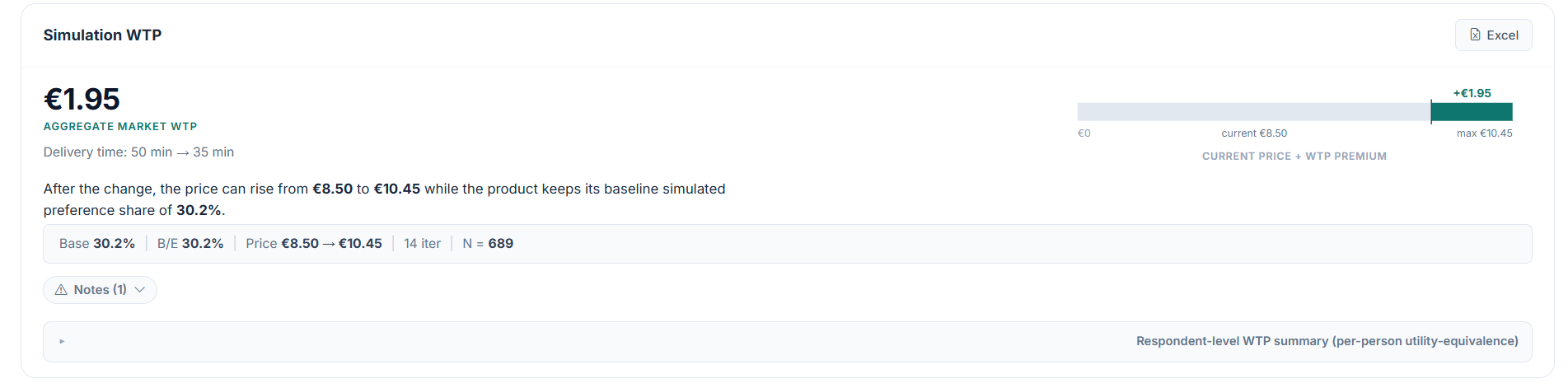
A worked example:
A negative WTP means the upgrade is actually a downgrade, consumers prefer the original level. A positive WTP means consumers value the upgrade and you could charge more for it.
Simulation WTP answers a positional question: "Given where my product currently sits in this market, what premium exactly offsets the attribute upgrade?" The answer genuinely depends on the focal product's starting price, and the direction of that dependence often surprises people.
An electricity-tariff study (price levels 45 to 65 EUR/month, three competing tariffs) tested the upgrade fossil fuel mix → renewable fuel mix on the focal tariff, once with the focal priced at 45 EUR and once at 65 EUR:
Intuition says the cheap product should have more "headroom", the simulation says the opposite. Neither number is a bug; they answer different questions.
Why this happens. In a market where every respondent had the same price sensitivity, the WTP would be identical at both starting prices (the utility gain divided by the price coefficient, see the proof in Section 10.3). With heterogeneous respondents, the break-even search is governed by whoever sits at the choice margin:
What to do instead:
"+7 EUR at a strong position" and "+53 EUR at a marginal position" are both mechanically correct answers to different positional questions. Only the in-range one is a defensible WTP estimate. When you need a single reportable number, use the mid-range setup or the SOS median, and state the focal price you used, because Simulation WTP is defined relative to it.
The Robust WTP sub-tab is described in the app as the recommended WTP approach. It extends Simulation WTP (Section 3) by removing the dependency on a specific set of competitor products. Instead of computing WTP against one fixed competitive scenario, it runs hundreds of Simulation WTP calculations, each with a different randomly generated competitive landscape. The result is a median WTP with bootstrap confidence intervals, a robust, scenario-independent estimate.
The panel description on the sub-tab reads: Sampling of Scenarios (SOS, Orme 2021), the recommended WTP approach. Does not use the products you set up under PRODUCTS. Instead, every scenario generates its own random competitive set and re-runs Simulation WTP for the selected attribute change. This stress-tests the WTP across many possible markets, so it does not depend on which competitors you happened to configure. The one exception is the Sample from products mode described in Section 4.3, which does draw from the PRODUCTS list.
SOS stands for Sampling of Scenarios (Orme, 2021). The idea: rather than relying on one particular competitive context (which may be arbitrary), sample many possible competitive contexts and report the central tendency.
Robust WTP is a wrapper around the Simulation WTP procedure. For each of N iterations:
After all iterations, the median WTP across all successful scenarios is reported together with two different measures of uncertainty:
The respondent bootstrap is used whenever the price attribute is linear, with or without the focal-product variations. Only when the run stores the price utility in a format that cannot be evaluated as a function of price does Choicery fall back to a resample of the scenario values, a Monte-Carlo interval of the scenario median that narrows with more iterations; the card then labels the row Scenario-resample 95% interval.
Exclude outliers works differently here than on the Simulation WTP sub-tab. With the setting on, scenario WTP values outside the P5 to P95 range of the scenario distribution are removed before the median, mean, confidence interval and SE are computed; more than 10 successful scenarios are required, otherwise the trim is skipped and the Notes say so. The Scenarios sheet of the Excel export marks such scenarios as not used and names the range.
Robust WTP repeatedly runs the same Simulation WTP procedure across many competitive scenarios. In the WTP tab, these inner Simulation WTP runs also use Share of Preference. Robust WTP does not switch to First Choice or Randomized First Choice.
The focal product is the product whose attribute you want to change, exactly as in Simulation WTP. You pick it in the shared Focal Product dropdown, and its levels come from the PRODUCTS panel. The competitors are always replaced per scenario; the focal product is only varied if you ask for it.
What the focal product determines:
Two checkboxes under the SOS controls change this. Also vary the focal-product price is on by default and varies the focal product's baseline price across the study price levels, so the estimate does not hinge on a single price anchor. Also test other focal-product level combinations is off by default and, when enabled, reruns each scenario across alternative valid combinations of the other focal-product levels while keeping the selected change fixed. Both are covered in Section 4.4.
The Mode dropdown controls how competitors are generated for each iteration:
| Mode | How It Works |
|---|---|
| Random from levels (default) |
For each competitor, independently samples one level per attribute from the study's design levels, uniformly at random. For example, with 3 body types, 4 colors, and 4 price levels, a random competitor might be Estate / Red / 30,000 EUR. Each competitor is generated independently.
If design prohibitions are active (e.g., “Economy brand cannot have 50,000 EUR price”), prohibited combinations are rejected and resampled. With conditional pricing, simulation retains the shared relative price levels estimated by HB. Brand-specific amounts shown in the survey do not replace those model levels. Results on this relative axis must not be interpreted as brand-specific willingness to pay in euros. |
| Sample from products | Draws K competitors from the products you have already defined in the PRODUCTS panel, excluding the focal product. If you have 5 products defined and the first one is focal, it samples from the remaining 4. Sampling is without replacement, so if K exceeds the number of available non-focal products, the scenario simply uses all of them. |
Click the Robust WTP sub-tab. The selection row stays where it is, the Calculate button is replaced by the SOS controls, and the panel description switches to the SOS text quoted above. Nothing is collapsed: Iterations, Competitors, Mode and Run SOS sit directly under the selection row, with the two focal-product checkboxes and the CSV checkbox below them.
The SOS controls on the Robust WTP sub-tab. They reuse the focal product and attribute change selected in the row above; the competitive set is regenerated per iteration.
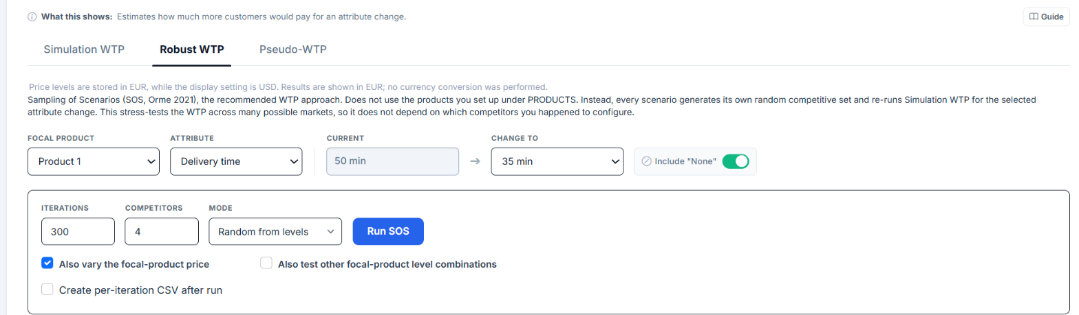
| Control | Default | Range | What It Does |
|---|---|---|---|
| Iterations | 300 | 10 to 2,000 | Number of random competitive scenarios to generate and evaluate. More iterations = more stable median but longer computation. |
| Competitors | 4 | 2 to 10 | Number of competitor products per scenario (K). Does not count the focal product itself. |
| Mode | Random from levels | - | How competitors are generated (see Section 4.3). |
| Also vary the focal-product price | on | on / off | When on, varies the focal product's starting price across iterations. Works independently of the level-combinations toggle, you can vary only the price while keeping the configured level combination fixed. On by default because the starting price is usually the strongest single influence on Simulation WTP (see Section 3.4). |
| Also test other focal-product level combinations | off | on / off | When on, varies the focal product's attribute-level configuration across iterations (instead of keeping it fixed). |
| Create per-iteration CSV after run | off | on / off | When enabled, the SOS run also writes a per-iteration CSV with the raw columns, meant for scripts. Choicery caches it temporarily and adds a CSV button to the result header. The file can be downloaded once: the button mints a download link that is valid for 60 seconds, and the cached file is removed after the download. The next Robust WTP run for the same analysis run replaces the cache. Nothing downloads automatically. The Excel export lists the scenarios either way, in its Scenarios sheet. |
Click Run SOS to start. A progress bar shows the running count of iterations and the percentage complete, and a Cancel button appears next to the run button while the job is running.
If you have active segment filters in the simulator (categorical or numeric), SOS runs the analysis for each segment separately, reporting per-segment median WTP with confidence intervals. Segment definitions that end up covering exactly the same respondents are computed once and reused, so the progress counter shows only the distinct runs.
The result card is headed Robust WTP (SOS) and carries an Excel button (and a CSV button when the per-iteration CSV was requested). The headline figure is labelled Median WTP for Change (SOS), next to two small histograms: the bootstrap distribution with the 95% CI marked, and the distribution of the scenario values with the P5-P95 band marked. Everything else sits in the meta row below it:
| Metric | Meaning |
|---|---|
| Median WTP for Change (SOS) | The central estimate, the median WTP across all successful scenarios. This is the primary number to report. The median is preferred over the mean because it is robust to extreme outlier scenarios. |
| Mean | The average WTP across scenarios. May be pulled by outlier scenarios; compare with the median. |
| Respondent bootstrap 95% CI | A nominal 95% confidence interval for SOS WTP in the target population: the median over the sampled competitive scenarios of their aggregate-market break-even WTP values, not the median of individual respondents' WTP values. It uses the percentiles of the per-draw medians from the respondent bootstrap (500 draws by default), keeping the competitive scenarios fixed while resampling respondents. Its repeated-study interpretation is that approximately 95% of intervals built this way would cover the corresponding population value, provided the bootstrap approximation is adequate. It is not a prediction interval for the next sample's estimate. On paths without the respondent bootstrap the row reads Scenario-resample 95% interval instead. |
| SE | The standard deviation of the bootstrap medians. Indicates precision of the median estimate. |
| Scenario band P5 to P95 | The 5th and 95th percentiles of the scenario WTP values. Not a confidence interval: it shows how much the competitive context moves the estimate. |
| scenarios | Number of successful iterations (scenarios where a valid WTP was found). Failed or boundary-estimate iterations are excluded. |
| Filtered respondents | Shown when a segment filter or the unusual-price exclusion reduced the respondent pool. |
| K | Number of competitors per scenario. |
| B | Number of bootstrap draws behind the interval (500 respondent draws by default; 2,000 scenario resamples on paths without the respondent bootstrap). |
| Mode | Echoes the competitor generation mode that produced the result: Random from levels or Sample from products. |
| Filtered respondents | Only shown when a segment filter was active. A chip next to the card title then names the segment and its n. |
Warnings, exclusion notices and the CSV note collapse behind the same Notes toggle as on the Simulation WTP sub-tab. If no scenario produced a usable estimate, the card shows the failure message instead of a value, and the CSV button stays available, because the per-iteration file is exactly what explains why everything failed. When at least one successful scenario placed the break-even price outside the tested price range, the Notes say how many of the scenarios did so. Those WTP values are extrapolations of the linear price effect; they stay in the median (Sawtooth reports the same share of extrapolated draws), the Excel Summary counts them, and the Scenarios sheet flags each of them.
When Also vary the focal-product price or Also test other focal-product level combinations is on, every scenario is evaluated for several versions of the focal product (different starting prices, or different level combinations). Within one scenario, Choicery runs the Simulation WTP search once per focal profile and takes the mean across those profiles as the scenario's WTP. The SOS headline is then the median over scenarios of these per-scenario means. So the nesting is: mean inside (over focal profiles), median outside (over competitive scenarios). The per-scenario detail (median and min-to-max range across the focal-product variations) is listed in the Notes of the Robust WTP card and in the Excel Summary.
Profiles whose search could not bracket a break-even price are not averaged in. They are counted and reported as profiles boundary in the Excel export and the result payload, next to the number of profiles used and the number skipped because they violated a design constraint. The mean over the remaining profiles is therefore a conditional mean: the average over those versions of the focal product whose break-even the search could reach. A high boundary count does not establish the direction of the difference from the full-profile mean. A lower-bound interpretation requires that the excluded profiles have finite WTP values at least as large as the retained mean; a boundary flag alone does not establish this. Extrapolation outside the tested price range is a separate case: if a break-even is found within the permitted search window, its WTP remains included and is flagged as extrapolated. Sawtooth's WTP report likewise flags extrapolated draws for cautious interpretation; that warning does not establish an identical rule for excluding boundary profiles.

The Excel export of a Robust WTP result has no Respondents sheet, because the headline is not a summary of individual values. In each scenario it is the price change at which the focal product’s share across all used respondents returns to its level before the change, and the card reports the median over the scenarios. People who hesitate between the focal product and its competitors and react to price move that share the most; people who choose it anyway, never choose it or barely react to price move it little. Neither the median nor the mean of the individual WTP values reproduces the headline, so the per-person values stay in the Simulation WTP export. The confidence interval on the card describes the median of the sample, not a single participant.
The Scenarios sheet lists every scenario: its WTP, whether it entered the median and, in plain words, why not, whether the break-even price lies outside the tested prices, the focal product’s share before the change, the starting and the break-even price, and one column per competitor. With active filters a Group column names the filter group. When the focal product is varied, share and prices are averages over the variations, and the Extrapolated column says in how many of them the break-even price lies outside the tested prices.
Interpretation: Across 287 different competitive scenarios (each with 4 random competitors), the median WTP for switching from SUV to Estate is −3,850 EUR. The negative sign means Estate is valued less than SUV, to maintain market share after switching to Estate, the price would need to decrease by approximately 3,850 EUR. The respondent bootstrap CI [−4,380, −3,290] shows how much the median would move with a different sample of people; the scenario band [−6,100, −1,900] shows how much the competitive context moves it.
The SOS median may differ from a Simulation WTP run because SOS samples across many competitive contexts. When both estimates agree closely, your WTP is robust to competitor assumptions. When they diverge, the WTP is sensitive to the competitive landscape, a valuable finding in itself. Switching sub-tabs does not discard either result: each sub-tab keeps its own last result, so you can flip between them and compare.
Click the Pseudo-WTP sub-tab. It uses a simple formula to convert utility differences into monetary amounts. It does not consider competitor products, it only looks at the utilities from the HB estimation. It is the sub-tab Choicery falls back to when the price-based methods are unavailable.
A thin bar at the top of the sub-tab shows the respondent count (N) and an info icon with the formula:
The default mode, selected with the left half of the pill toggle above the form (Attribute Change / Product Comparison). Select an attribute, the current level and the target level. Choicery computes the WTP for this single attribute change, holding everything else constant.
| Control | Example |
|---|---|
| Attribute | Color |
| Current | White |
| Change to | Red |
Click Calculate to see the WTP result across all respondents.
Switch the pill toggle to Product Comparison. There is nothing to select here: the note in the form states that it compares Product 1 → Product 2 from the Products panel, and that all attribute values except price are taken from there automatically. Choicery then computes the total WTP difference between the two profiles, summing the utility differences across all attributes. Edit the two products in the PRODUCTS panel if you want to compare a different pair.
The headline figure is labelled Median Pseudo-WTP whenever the WTP divides by each respondent's own price coefficient, that is for a linear and for a categorical price (see the box below for why). Only with a manual conversion factor, which applies one factor to everyone, is it the Mean Pseudo-WTP. It sits next to a small spread graphic marked respondent spread, P5-P95. Underneath it, three stat tiles (the other central statistic, Std Dev, P5-P95) and a context line naming the attribute change; the N in the formula bar is the number of respondents that entered the statistics:
| Metric | What It Tells You |
|---|---|
| Mean | Average across all respondents. Can be distorted by outliers: a few respondents whose price coefficient is just above the near-zero screen produce very large values and lift the mean. |
| Median | The middle value. More robust, always prefer this for reporting. |
| Std Dev | How much WTP varies across respondents. Large SD = high preference heterogeneity. |
| P5-P95 (respondents) | The range covering the central 90% of individual-level WTP values (5th to 95th percentile). This is a spread across people, not a confidence interval. Inspect it for outliers or wide preference heterogeneity. |
As on the other sub-tabs, exclusion and trimming notices collapse behind a Notes toggle. With Include unusual price responses on, the Notes say how many respondents who seem to prefer higher prices or barely react to price were kept; their values can be very large or have the opposite sign. If the price attribute was not estimated as linear and you entered a conversion factor by hand, the result additionally carries a Manual Mode badge.
When price was estimated as categorical, there is no single price coefficient. Choicery then fits, for each respondent, a least-squares line through that respondent's utilities of the price levels against the numeric price values of the levels: the values you entered via Set values for all levels, or, if you did not, the numbers contained in the level labels (enter all levels when the labels are not numeric). The slope of that line is the respondent's price sensitivity in utility per currency unit, and the respondent's Pseudo-WTP is the utility difference of the attribute change divided by the absolute slope. This is the same fit that Reservation Price uses, so both analyses now rest on the same individual price slopes. The conversion factor shown in the Price Configuration panel is the pooled reference line through the mean utilities; it is only used for the calculation itself when no individual slope is usable, and the result then says so in its notes.
Because the slopes are individual, the same screening as for a linear price applies: respondents whose slope is positive (they seem to prefer higher prices) or near zero (their utility moves by less than 0.1 over the whole tested price range) are excluded unless Include unusual price responses is on. The Notes list how many were removed for each reason.
The headline is the Median Pseudo-WTP in this mode. Dividing by an individual slope makes the mean fragile: a respondent whose slope is small but just above the screening threshold produces a WTP several times the typical value, and a few such cases move the mean by a large amount while the median barely reacts. In a synthetic check with four price levels the medians of the pooled and the individual variant agreed within 2 to 3%, while the mean of the individual variant was two to three times larger. Orme (2020) describes exactly this: near-zero price coefficients make “the dollar equivalents for incremental features … very large, approaching infinity. A typical way to handle this is to characterize the centers of the distributions using medians rather than means.” The mean, Std Dev and P5-P95 stay on the card so you can see how wide the individual distribution is.
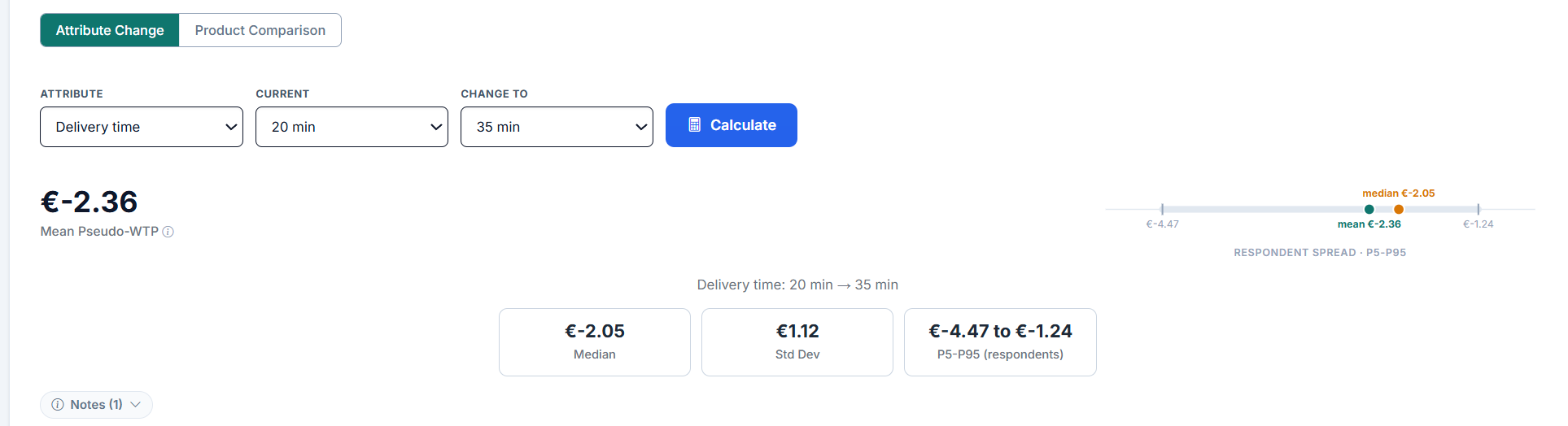
Interpretation: The median respondent would pay about 7,400 EUR more for a red car than a white one, all else being equal. Use the median for reporting.
If you see very large WTP values (e.g., >100,000 EUR for a color change), this usually means some respondents have near-zero price coefficients (they ignored price in the survey). The median is much more reliable than the mean in this case. See the Attribute Non-Attendance section in Part II for details.
| Scenario | Method | Why |
|---|---|---|
| Default for most studies | Robust WTP (SOS) | Robust across many competitive scenarios. Reports confidence intervals. Not dependent on any single competitor configuration. |
| Industry study with well-defined, stable competitors | Simulation WTP | Accounts for a specific competitive landscape. Useful when you know exactly who the competitors are. |
| Stakeholder presentation requiring confidence intervals | Robust WTP (SOS) | The bootstrap CI gives a credible uncertainty range. Harder to challenge than a single point estimate. |
| Academic research on consumer preferences | Pseudo-WTP | Standard in academic literature. No competitors needed. Report the median. |
| Quick screening before deep analysis | Pseudo-WTP | Fast, no product setup required. Good for initial exploration. |
| All competitors are basically identical | Either (results are the same) | When competitors are identical, Simulation WTP mathematically reduces to Pseudo-WTP (see Section 10). |
| Study has no price attribute | Pseudo-WTP, Manual Mode only | Choicery offers a hand-entered conversion factor (1 utility unit = X) and flags the result Manual Mode. It assumes the same price sensitivity for everyone; use it for exploration, not for reporting. Attribute Importance is the better summary. |
Academic foundations, formulas, and methodological details behind WTP estimation.
These concepts are related but distinct (Orme, 2020, Section 9.6). WTP measures consumer valuation. Price sensitivity measures consumer reaction. Price elasticity measures market-level demand response. MVAI measures firm pricing power.
The simplest and most widely used WTP method in conjoint analysis. It converts utility differences into monetary units by dividing by the price coefficient. Allenby et al. (2014) explicitly term this "pseudo-WTP" to distinguish it from the formal welfare-theoretic WTP measure.
Where βprice is the linear price coefficient (a single parameter). Using linear price coding yields a consistent conversion factor regardless of how many price levels exist in the design.
With three or more categorical price levels, Choicery does not pick two levels for Equation 9.1. It fits a least-squares line through all (price value, utility) points of each respondent and uses that respondent's slope as βprice in Equation 9.3. With exactly two levels the line passes through both points and the two formulas coincide. This is the same per-respondent line that Reservation Price uses.
A study examines willingness to pay for renewable vs. fossil energy sources.
Interpretation: On average, consumers would pay 18 EUR/month more for renewable energy compared to fossil energy, holding all other attributes constant.
Orme (2020) and Allenby et al. (2014) identify several fundamental problems, ranked by severity:
| # | Problem | Description |
|---|---|---|
| 1 | Ignores competition | Most fundamental flaw. WTP is computed as if no alternative products exist, the "Gilligan's Island" problem (see Section 14). Orme (2020) considers this the single biggest limitation. |
| 2 | No specific product | The ratio considers an "average product" rather than a defined competitive offering. |
| 3 | Market average only | Reports average WTP across all respondents rather than for the target segment. |
| 4 | Reversed price signs | Positive price coefficients (estimation noise) create nonsensical negative WTP. |
| 5 | Near-zero denominators | Very small price coefficients cause WTP to approach infinity. Common with respondents who ignored price (ANA, see Section 16). |
| 6 | Non-linear price utility | With 3+ categorically coded price levels, there is no single "price coefficient," making the conversion factor ambiguous. |
| 7 | Hypothetical bias | Respondents spend "survey dollars" more freely, making price utilities too small and inflating WTP (see Section 15). |
| 8 | Attribute non-attendance | Respondents who ignore price produce extreme WTP outliers (see Section 16). |
Despite its limitations, the simple ratio method remains the standard approach in academic research when the research question is about consumer preferences rather than firm pricing. It is appropriate when:
Originally proposed by Orme (2020, Section 9.6; Orme & Chrzan, 2017, Ch. 13) as the preferred method. Instead of dividing utilities by a price coefficient, this method uses the market simulator to find the price increase that exactly offsets a feature improvement's share gain. Section 11 extends this to multiple randomized scenarios (SOS Bootstrap).
This is Orme's strongly preferred approach. It accounts for the full competitive landscape. The underlying algorithm performs these steps automatically:
In a logit model with identical competitor products, simulated WTP equals pseudo-WTP regardless of the number of competitors. The number of identical alternatives cancels out in the logit probability ratio.
Proof sketch: In a logit model, the choice probability for product j is:
With N identical competitors (each having utility Vc) and one focal product with utility Vf:
The simulated WTP procedure finds the price change Δp such that the focal product's share returns to its baseline after adding a feature with utility δ. Setting the shares equal:
Since the structure is identical on both sides, the N cancels, and the solution is simply Δp = δ / βp, exactly the pseudo-WTP formula. This means that for studies where competition is identical or undefined, the simple ratio method is mathematically equivalent.
The identical-competitors proof above has an important corollary: in a homogeneous logit market, the break-even price increase is Δp = δ / βp regardless of the focal product's starting price or baseline share. The starting position cancels out exactly the way N did.
With heterogeneous respondents this invariance breaks. The aggregate Share of Preference is a mixture of individual logit shares:
The break-even search solves S(p₀ + Δp | upgraded) = S(p₀ | baseline). Because each respondent's share contribution saturates at a different rate, the solution Δp depends on which respondents are near their choice margin at p₀:
Two practical consequences follow:
This is the same class of aggregation phenomenon that Ofek & Srinivasan (2002) address with MVAI (Section 12): monetizing an attribute change at the market level requires weighting respondents by their marginal impact on share, and that weighting depends on the market position at which it is evaluated. SOS Bootstrap (Section 11) mitigates, though does not remove, position dependence by averaging over many competitive contexts and, optionally, focal configurations.
Standard Simulation WTP (Section 10) computes the price a firm could charge for an attribute improvement in a specific competitive scenario. But this raises a question: how sensitive is the WTP estimate to the particular competitors chosen?
Orme (2021) addresses this with Sampling of Scenarios (SOS): instead of computing WTP in one fixed competitive context, run the procedure across many randomly sampled competitive contexts and report the median WTP as a robust, scenario-independent estimate.
In practice, researchers often face uncertainty about which competitors to include. Different competitor configurations can produce materially different WTP estimates. SOS addresses this by:
The median is used instead of the mean for two reasons:
The confidence interval is estimated using the percentile bootstrap method (Efron & Tibshirani, 1993). The procedure:
Only when the respondent bootstrap is unavailable does Choicery resample the scenario values instead (B = 2,000, labelled Scenario-resample 95% interval).
The SOS confidence interval reflects sampling uncertainty over respondents: how much the SOS median would move with a different sample of people from the same population. How much the competitive context moves the estimate is shown separately by the scenario band P5 to P95: a wide band means the competitive landscape matters a lot for this attribute, in itself a useful insight for pricing strategy.
When generating random competitors in “Random from levels” mode, Choicery respects the study's design constraints:
Not every scenario yields a valid WTP. Two types of non-results are tracked:
| Type | Cause | Treatment |
|---|---|---|
| Boundary estimate | The binary search could not find a price at which the focal product's share returns to baseline (the price would need to be extremely high or low). | Excluded from the WTP distribution. Reported as “N iterations returned boundary estimates (break-even not found) and were excluded.” |
| Failed iteration | The simulation encountered an error (e.g., all competitors had identical utility, numerical issues). | Excluded. Reported as “N of M iterations failed and were excluded.” |
If all iterations fail, Choicery reports “All iterations failed. Check your product configuration.”, typically indicating a problem with the price attribute setup or the focal product definition.
| Method | Competitive Context | Uncertainty Quantification | Speed |
|---|---|---|---|
| Pseudo-WTP | None (ignores competition) | None (single point estimate) | Instant |
| Simulation WTP | Fixed (user-defined competitors) | None (single point estimate) | Fast (<1 second) |
| Robust WTP (SOS Bootstrap) | Randomized (many scenarios) | Bootstrap CI + SE on the median | Moderate (seconds to minutes, depending on iterations) |
Use Pseudo-WTP for quick screening. Use Simulation WTP when you have a well-defined, stable competitive landscape. Use Robust WTP for most studies, it provides robustness to competitor assumptions and confidence intervals.
Developed by Ofek & Srinivasan (2002), MVAI provides a theoretically grounded, closed-form expression for the market's value of a product attribute improvement. It answers: "How much more could a firm charge for an attribute improvement while keeping market share constant?"
MVAI is defined as the ratio of the change in market share due to an attribute improvement to the change in market share due to a price increase (Ofek & Srinivasan, 2002, Eq. 7):
In words: the incremental price that maintains constant market share after an attribute improvement. This is equivalent to the Simulated WTP concept (Section 10.2) but derived analytically.
Using the multinomial logit framework with individual-level parameters, Ofek & Srinivasan (2002, Eq. 14) derive:
where the customer weights ai are:
Here:
wik = individual i's utility weight for attribute kwip = individual i's price sensitivityθji = individual i's probability of choosing firm j's productμi = individual i's logit scale parameter (inversely related to error variance)qi = individual i's maximum purchase quantityThe factor θji(1 − θji) is a concave function that peaks at θ = 0.5 and approaches zero as θ → 0 or θ → 1. This means:
Ofek & Srinivasan (2002) note the analogy to political campaigns: effort is best spent on undecided voters.
The standard practice (Orme, 2001; Wyner, 1997) is to average individual WTP ratios wik/wip across respondents. Ofek & Srinivasan (2002) show this differs substantially from MVAI:
| Property | MVAI (Eq. 12.2) | Average Ratios |
|---|---|---|
| Structure | Ratio of two sums | Sum of individual ratios |
| Customer weighting | θ(1−θ) weighting + μi scale | Equal weight (or quantity-weighted) |
| Sensitive to competition? | Yes (θ depends on competitive set) | No (only individual parameters) |
| Outlier robustness | High (extreme wip damped by θ(1−θ)) | Low (near-zero wip explodes) |
| Empirical divergence | Averages differed from MVAI by 101.4% (Table 2, Ofek & Srinivasan, 2002) | |
MVAI answers a firm-centric question ("How much more can a specific firm charge?"), not a consumer-centric one ("How much do consumers value this feature?"). For academic WTP research without a specific firm context, the simple ratio method may be more appropriate. MVAI is documented here for theoretical context and comparison with the implemented WTP workflows.
Allenby, Brazell, Howell, and Rossi (2014) argue that the only sensible metric for assessing a product feature's value to a firm is its impact on profits. They define the economic value of a feature enhancement as:
where A* is the market with the enhanced product and A is the market without it, both evaluated at their respective Nash equilibrium prices.
Allenby et al. (2014) make two key critiques:
Their formal WTP measure, derived from the indirect utility function (Eq. 2.12):
This method is documented here for theoretical context and comparison with the implemented WTP workflows.
Both Orme (2020) and Orme & Chrzan (2017) use this parable to illustrate the fundamental flaw of WTP without competition:
Rich castaways stranded on a desert island would pay virtually any amount for rescue when only one boat arrives. Their WTP for the boat is astronomical, potentially their entire net worth.
But when a second boat arrives offering rescue for $5,000, the WTP for the first boat drops to approximately $5,000.
Lesson: Without competition, WTP equals the "maximum price" a consumer would pay, which can be astronomical. In competitive markets, actual WTP is bounded by alternatives.
Computed WTP for a color monitor over monochrome would be $1,000+ based on utility ratios. But color monitors are readily available at inexpensive prices. The WTP number is meaningless because it ignores that every competing laptop already has a color screen.
The Gilligan's Island problem is most severe when the feature being valued has no close substitutes or when competition is not modeled. For studies measuring WTP for features that are widely available, the competitive context naturally bounds the estimate and pseudo-WTP may be acceptable.
Respondents consistently spend "survey dollars" more readily than real ones. This makes price utilities too small (respondents appear less price-sensitive than they actually are), which inflates WTP (Orme & Chrzan, 2017, Ch. 2 and 13).
| Remedy | Mechanism | Evidence |
|---|---|---|
| None/opt-out alternative | Realistic opt-out reduces forced choice inflation | Widely recommended (Allenby et al., 2014) |
| Cheap talk scripts | Tell respondents that past surveys show overstatement | Mixed evidence (Fifer et al., 2014) |
| Certainty scales | Ask confidence after each task; discard low-certainty | Effective for binary WTP (Loomis, 2011) |
| Budget constraint reminders | Remind respondents of their real-world budget | Reduces hypothetical bias modestly |
| Incentive alignment | Real monetary consequences for survey choices | Gold standard (Ding, Grewal, & Liechty, 2005; Sablotny-Wackershauser et al., 2024) |
| Adaptive designs (ACBC) | Tailored tasks improve engagement and realism | Sablotny-Wackershauser et al. (2024) show ACBC reduces bias |
| RP/SP data fusion | Combine stated preference with revealed preference data | Calibrates hypothetical responses against real behavior |
Crossing incentive alignment mechanisms with adaptive conjoint designs (ACBC) can improve WTP estimation. The "inferred WTP" mechanism, where the design adapts to find the participant's indifference price, provides more precise individual-level WTP estimates than standard CBC, but requires careful implementation to avoid strategic responding.
When respondents completely ignore the price attribute during choice tasks, their estimated price coefficient approaches zero. Dividing by a near-zero price coefficient produces enormous WTP values (approaching infinity). This is a major source of WTP outliers (Orme, 2001; Hensher, Rose, & Greene, 2005).
WTP can be estimated at three levels of granularity:
| Level | Method | Output | When to Use |
|---|---|---|---|
| Aggregate | Single model for entire sample | One WTP value | Quick screening, presentations |
| Segment-level | Latent class (LC) analysis | Discrete set of WTP values per class | Market segmentation, targeting |
| Individual-level | HB or mixed logit | Nearly continuous distribution | Full distribution analysis, precision |
The field is moving toward individual-level WTP, considering the full distribution rather than a single point estimate. Sampling from HB posterior draws gives a more complete picture (Orme & Chrzan, 2017, Ch. 13). Best practice is to report both the median (robust to outliers) and the distribution (histogram or kernel density).
Allenby, G. M., Brazell, J. D., Howell, J. R., & Rossi, P. E. (2014). Economic valuation of product features. Quantitative Marketing and Economics, 12(4), 421-456. doi:10.1007/s11129-014-9150-x
Berry, S. T. (1994). Estimating discrete-choice models of product differentiation. RAND Journal of Economics, 25(2), 242-262.
Ding, M., Grewal, R., & Liechty, J. (2005). Incentive-aligned conjoint analysis. Journal of Marketing Research, 42(1), 67-82.
Efron, B., & Tibshirani, R. J. (1993). An introduction to the bootstrap. New York: Chapman & Hall.
Fifer, S., Rose, J., & Greaves, S. (2014). Hypothetical bias in stated choice experiments: Is it a problem? And if so, how do we deal with it? Transportation Research Part A: Policy and Practice, 61, 164-177.
Hensher, D. A., Rose, J. M., & Greene, W. H. (2005). Applied choice analysis: A primer. Cambridge: Cambridge University Press.
Loomis, J. (2011). What's to know about hypothetical bias in stated preference valuation studies? Journal of Economic Surveys, 25(2), 363-370.
McFadden, D. (1974). Conditional logit analysis of qualitative choice behavior. In P. Zarembka (Ed.), Frontiers in econometrics (pp. 105-142). New York: Academic Press.
Ofek, E., & Srinivasan, V. (2002). How much does the market value an improvement in a product attribute? Marketing Science, 21(4), 398-411.
Orme, B. K. (2001). Assessing the monetary value of attribute levels with conjoint analysis: Warnings and suggestions. Conjoint Analysis Customer Newsletter (Spring). Sequim, WA: external conjoint software
Orme, B. K. (2020). Getting started with conjoint analysis: Strategies for product design and pricing research (4th ed.). Manhattan Beach, CA: Research Publishers LLC.
Orme, B. K. (2021). Getting started with conjoint analysis: Strategies for product design and pricing research (5th ed.). Manhattan Beach, CA: Research Publishers LLC.
Orme, B. K., & Chrzan, K. (2017). Becoming an expert in conjoint analysis: Choice modeling for pros. Orem, UT: Commercial conjoint software publisher
Revelt, D., & Train, K. (1998). Mixed logit with repeated choices: Households' choices of appliance efficiency level. Review of Economics and Statistics, 80(4), 647-657.
Sablotny-Wackershauser, V., Lichters, M., Guhl, D., Bengart, P., & Vogt, B. (2024). Crossing incentive alignment and adaptive designs in choice-based conjoint: A fruitful endeavor. Journal of the Academy of Marketing Science, 52(3), 610-633.