How to estimate the maximum price consumers would pay for a product configuration, a practical guide for Choicery with methodological background.
Everything you need to estimate, interpret, and export Reservation Prices in Choicery.
The reservation price is the maximum price a consumer would pay for a specific product before choosing not to buy at all (or switching to a competitor). At this price, the consumer is exactly indifferent between buying and not buying.
Unlike WTP (willingness to pay), which measures the value of changing a single attribute level, the reservation price evaluates a whole product configuration. It answers a fundamentally different question:
“For an SUV in Red at the Premium trim level, what is the maximum price consumers would accept?”, This is a reservation price question. It prices an entire product bundle, not a single feature upgrade.
WTP asks: “How much more would a consumer pay to upgrade from Level A to Level B?” It measures the incremental value of an attribute change. Reservation Price, by contrast, asks: “What is the absolute maximum price for this complete product?” It integrates all attribute utilities into a single price figure. Section 12 provides a detailed comparison.
Use Reservation Price when you need to set or evaluate the actual price of a specific product configuration, for launch pricing, price testing, or demand estimation. Use WTP when you need to understand the relative value of individual features.
Before using Reservation Price in Choicery, ensure the following are in place:
A completed HB estimation with individual-level utilities. Reservation Price requires individual part-worth utilities (one set per respondent). Run HB estimation first in the Analysis tab.
A price attribute. Your conjoint design must include a price attribute. Linear coding is preferred for the most reliable reservation prices. Categorical (part-worth) coding also works but produces an approximation via OLS interpolation (see Section 9.3).
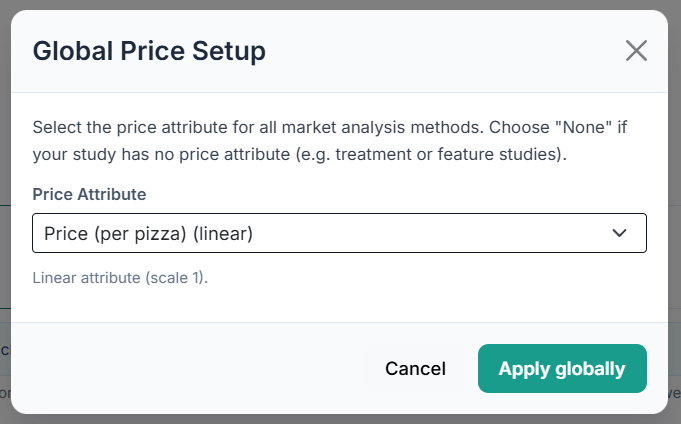
Price Setup completed. The price attribute is set once for all price-based methods through the Price Setup button in the top bar, which opens the Global Price Setup dialog. Pick the attribute in Price Attribute; for a categorical price attribute the dialog also lists every level under Enter numeric values for categorical price levels. Values are prefilled from the level labels where they can be parsed; fill in or adjust them so that every level has a value and at least two values differ. Confirm with Apply globally. Until a price attribute is selected, the Reservation Price tab shows “Choose a price attribute first in Price Setup (top bar) to enable this method.” and stays disabled.
Ideally: HB estimation with a None option included. The None option provides the outside good utility (Voutside), which is needed for absolute reservation prices. Without it, results are relative reservation prices (still useful for comparisons, but not an absolute maximum price). See Section 5 for a detailed discussion.
If your conjoint design did not include a None option, Choicery will set Voutside = 0 and display a warning. The resulting reservation prices are relative, useful for comparing configurations, but not interpretable as an absolute maximum price.
The Reservation Price tab has no attribute editor of its own. It reads the first product in the PRODUCTS panel on the left of the Market Simulator, and every further product in that panel is treated as a competitor. If you want to price a different configuration, edit the first product in the PRODUCTS panel and press Calculate again.
Above the Calculate button the tab shows only a caption: “Calculating reservation price for Product 1 from the Products panel. Edit it there to change the configuration.” The bold part is the product’s own name, so it changes if you renamed the product. Notice that the price attribute is the one being solved for, so the price level you set on the first product is dropped before the calculation. The Reservation Price calculation determines at what price point each respondent would be indifferent between buying this configuration and taking the best alternative.

Every product after the first one in the PRODUCTS panel is automatically sent along as a competitor and acts as a competitive floor. The reservation price becomes the price at which a consumer would switch to the best available alternative (not just the outside option). See Section 4.2.
The respondent-filter policies are shared across the price methods and live in the top-bar Analysis Settings menu (header: Shared analysis policies). The Reservation Price tab itself only carries the bootstrap seed, behind its Advanced Settings toggle just below the Calculate button.
| Option | Where | Default | Description |
|---|---|---|---|
| Include unusual price responses in price analyses | Analysis Settings | OFF | Some respondents show price-quality inference (higher price = higher utility) or barely react to price across the studied price range. Including them can produce negative or extreme RPs. Default exclusion is recommended. The same switch applies to WTP, Price Elasticity and Sensitivity on price; Choice Share always uses all respondents. |
| Exclude outliers | Analysis Settings | OFF | Outliers are identified via the Tukey IQR method (below Q1 minus 1.5 times IQR or above Q3 plus 1.5 times IQR). Turn this on when extreme RPs should be removed from summary statistics. The same switch can be flipped from the result view, see Section 4.1. |
| Allow negative prices | Analysis Settings | OFF | Applies to WTP and Price Elasticity only. Reservation Price is not affected: it always computes negative values and has its own display toggle (Section 4.3). |
| Bootstrap seed | Advanced Settings (RP tab) | 1 | Random seed for the bootstrap confidence interval resampling. The default 1 is the shared simulation seed used by every stochastic tab, so the same seed gives the same result across tabs. Change it only for reproducibility checks. The bootstrap uses 1,000 resamples in all cases. |
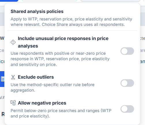
If a large proportion of respondents have unusual price responses, this may indicate a model issue (e.g., price was not varied enough, or respondents used price as a quality signal). Consider revisiting HB settings, sign constraints on the price coefficient can help.
Click Calculate. No new estimation is started: the request only re-uses the individual-level utilities from the existing HB run, so the results come back within a moment. If the PRODUCTS panel is empty, Choicery warns “Add at least one product in the Products panel, Reservation Price uses Product 1.”. If filters are active in the left panel, the segmented demand curve is calculated in the same step.
The results panel opens with the heading Results, an Excel download button on the right, and four summary cards: Median RP, Mean RP, 95% CI (Mean) and N used.

Below the demand curve, a line summarises which respondents were dropped or kept, for example “Excluded: 12 unusual price responses (7 prefer higher prices, 5 barely react to price)”. When outliers exist, an inline Exclude outliers / Include outliers button sits next to that line and re-runs the calculation with the flipped setting, so you do not have to open the Analysis Settings menu.
Directly below the statistics cards, a contextual note states the competitive setup:
When competitors are present, the RP threshold uses max(V_outside, best_competitor_utility). This means the reservation price is the price at which a consumer would switch to the best available alternative, whether that is not buying at all or buying a competitor product.
Without competitors, the RP threshold is only the outside option (None). This may overestimate the reservation price, the classic “Gilligan’s Island” problem. On a deserted island with no alternatives, consumers would pay almost any price. In real markets, competitors constrain pricing.
By default, Choicery displays capped reservation prices: any negative RP is set to zero. This makes practical sense, a negative price means you would have to pay the consumer to accept the product. A note above the demand curve states the current mode, for example “Showing values capped at €0 (default). 14 respondents below €0 are counted at €0 and stay in N. This leaves the median unchanged and lowers the mean.” In the raw view it reads “Showing raw values (including negative reservation prices).”
Clicking Show negative values (the link turns into Hide negative values) reveals the raw distribution, including negative RPs. A negative reservation price means the consumer values the product less than not buying, they would need to be compensated to accept it. This is useful for diagnostic purposes: a large cluster of negative RPs suggests the product configuration is deeply unattractive to a segment of the market. The toggle switches all four cards and the segment table between the capped and the raw statistics; the 95% CI (Mean) is bootstrapped separately on each version.
The demand curve is the most powerful output of Reservation Price analysis. It shows the percentage of respondents willing to buy at each price point. The chart header carries a PNG button that saves the plot as a high-resolution image. The caption in the app reads: “Percentage of consumers willing to buy at each price point. The x-axis is capped to the studied price range when available; demand may remain above 0% at the highest tested price.”
How to read the demand curve:
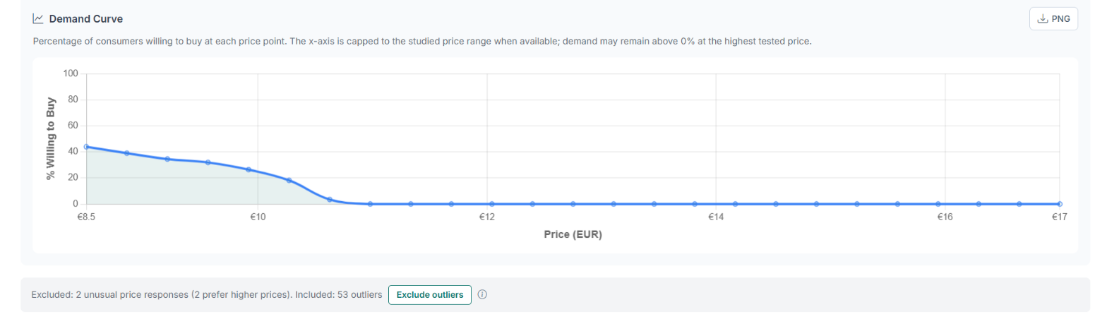
A single number (median RP) hides the distribution. Two products might have the same median RP but very different demand curves, one with a tight distribution (homogeneous market, clear price point) and another with a wide spread (heterogeneous market, segmentation opportunity). Always inspect the curve.
When filters are active (the Filters button at the top of the left panel), the demand curve shows the full sample as a dashed grey Overall line and one colored line per segment, labelled with the segment name and its n, on a shared price axis. A legend appears only in this segmented view. Medians are not marked on the chart; read them from the segment table above it. This immediately reveals which segments have higher price tolerance. Segments that cannot be evaluated are reported as “Segment curves: N plotted, M skipped”.
When filters are active, a segment table appears between the context note and the demand curve. Its heading follows the segment count: with one segment it reads Reservation Price: Overall vs <segment name>, with several segments Reservation Price: Overall vs Segments. Its columns are Segment, n, Median, Mean and 95% CI, and the first row is always the full sample:
| Segment | n | Median | Mean | 95% CI |
|---|---|---|---|---|
| Overall | 287 | €34,250 | €36,480 | €32,100 - €36,400 |
| Premium Seekers | 94 | €41,200 | €43,150 | €38,900 - €43,500 |
| Value Shoppers | 112 | €28,750 | €29,400 | €26,800 - €30,700 |
| Brand Loyalists | 81 | €35,600 | €36,200 | €33,100 - €38,100 |
From two segments upwards, the highest and the lowest median are colour-marked (here: Premium Seekers and Value Shoppers), so the most and least price-tolerant customer group for this product configuration are visible at a glance. If the medians are all identical, no marking is applied. Segments that could not be computed are listed below the table as “Skipped segments: …”.
This distinction is critical for interpreting reservation prices correctly.
Whether your reservation prices are absolute or relative depends entirely on whether the HB estimation included a None option. The numbers may look similar, but their interpretation is fundamentally different.
When the HB estimation includes a None option (a “no-buy” alternative in each choice task), the model estimates an individual-level utility for the outside good: Voutside. The reservation price is the price at which the product’s utility equals Voutside, making this a true indifference price.
This is the gold standard. The result can be interpreted as: “At this price, the consumer is exactly indifferent between buying this product and walking away.”
Without a None option, there is no estimated outside good utility. Choicery sets Voutside = 0, which acts as a neutral baseline. The resulting reservation price is relative, it measures the price at which the product’s utility equals zero, not the price at which the consumer would actually stop buying.
“No None-Option was included in HB estimation. Using V_outside = 0 as baseline. This provides ‘relative’ reservation prices. For true absolute reservation prices, re-run HB with None-Option enabled.” This footnote appears at the bottom of the tab when no None utility is available, with an information icon on the phrase “V_outside = 0”. A second variant, “None-Option is enabled in the analysis run, but respondent-level None utilities are missing…”, appears when the run says it used a None option but the individual None utilities cannot be found. In both cases the numbers are still useful for comparing product configurations (which one has a higher RP?), but they should not be presented as absolute maximum prices.
Always include a None option in your conjoint design if you plan to use Reservation Price analysis. This is standard practice in CBC (Orme, 2020) and provides the reference point needed for absolute pricing insights.
Click the Excel button in the Results header to export a workbook named reservation_price_YYYYMMDD_HHMMSS.xlsx. The export reuses exactly the result that is on screen, so calculate first. The following sheets are written; the segment sheets only appear when filters were active:
| Sheet | Contents |
|---|---|
| Summary | Metric and value pairs: price attribute and currency, then mean, median, standard deviation, the 5th / 25th / 75th / 95th percentile, minimum, maximum, the two 95% CI bounds, the bootstrap standard error, total and valid respondents, the unusual-price-response counts (total, excluded, included), the number of detected outliers (row “Excluded (Outliers)”, reported whether or not the outlier switch was on), the number of competitors in context, and the bootstrap seed. Below that, a second block lists the product configuration as Attribute and Level. |
| Individual_RP | One row per respondent with the columns Respondent, Reservation_Price and Valid. Respondent carries the original respondent identifier where a respondent mapping exists. Reservation_Price is empty for respondents that were excluded, and Valid is then FALSE. |
| Demand_Curve | Columns Price, Demand_Pct and Respondent_Count for the overall curve, ready for charting in Excel or other tools. |
| Segment_Demand_Curves | The same three columns per price point, prefixed with a Segment column, one block per plotted segment. |
| Extended_Demand_Curves | Export-only curves on a wider shared price axis that spans the studied price range, the central 90 percent of the overall reservation prices, and every visible segment median. Columns: Series (Overall or segment name), Price, Demand_Pct, Respondent_Count and Range_Status, where Range_Status is Studied inside the tested price levels and Extrapolated outside them (Modeled if the studied range could not be resolved at all). Use this sheet when you need demand beyond the tested price levels, and treat the Extrapolated rows accordingly. |
| Warnings | The methodological warnings shown in the tab (missing None option, unusual price responses, price attribute override). |
| Segment_Summary | Per-segment statistics: Segment, Respondents, Valid_Respondents, Mean, Median, Std, Percentile_5, Percentile_95, CI_Lower, CI_Upper. |
| Segment_Errors | Segments that were skipped, with the reason. |
| Segment_Definitions | The filter definitions behind the segments, so the export documents how each segment was cut. |

The PDF button at the right end of the tab bar renders a report for the tab that is currently open, so with the Reservation Price tab active you get a Reservation Price report containing the statistics and the demand curve. It uses the result that is currently displayed, so calculate before exporting; otherwise Choicery reports “Calculate this analysis again before exporting its PDF.”
1. Is the None option included? (absolute vs. relative) 2. Are competitors defined? (competitive context) 3. Is the price attribute linear? (reliability) 4. How many respondents were excluded? (sample representativeness) 5. What does the demand curve look like? (distribution shape)
The mathematical foundations, formulas, and methodological nuances behind Reservation Price estimation.
max(V_outside, best_competitor_utility). The reservation price is the price at which the focal product’s utility equals this threshold.When the price attribute is coded linearly in the HB estimation, each respondent n has a single price coefficient βprice(n). The reservation price is derived by solving for the price at which the product’s total utility equals the threshold utility:
Where:
max(V_outside, max_competitor_utility), the best alternative available to the consumer.The numerator measures how much non-price value the product offers above the best alternative. The denominator converts this utility surplus into a price unit. A larger surplus or a less price-sensitive consumer (smaller |βprice|) yields a higher reservation price.
Because Julia/HB estimates the price coefficient on centered and scaled price values (to improve MCMC convergence), the raw RP from Equation 1 must be corrected:
Here, price_mean is the centering value used when the run was estimated. For HB runs this is the arithmetic mean of the price levels in the design (the Julia sampler also divides by half the price range for MCMC stability); for AI-Driven Profile Analysis runs it is the standardization mean stored with the run. The rp_delta represents the price deviation from this mean that would make the consumer indifferent. Adding it back to the mean yields the actual reservation price in the original currency unit.
When the price attribute uses categorical (part-worth) coding, there is no single price coefficient. Instead, each price level has its own utility. To derive a reservation price, Choicery uses an OLS regression of the level utilities on the price values to estimate a pseudo-linear price coefficient per respondent. The numeric price value behind each level is the value confirmed in the Global Price Setup dialog (Section 2); Choicery prefills those fields from the level label where it can be parsed, and you can adjust them before applying. Both the fitted slope and the fitted intercept are used when solving for the indifference price, and no centering term is added, because the regression is run on the raw price values.
This approach assumes that utility is approximately linear in price for each individual, which may not hold. The resulting RPs should be treated as exploratory. For actionable pricing decisions, use linear price coding in HB.
Consider three respondents evaluating an “SUV · Red · Premium” configuration. The price mean is €30,000.
| Respondent | Vproduct | Vthreshold | βprice | rp_delta | RP |
|---|---|---|---|---|---|
| Alice | 3.20 | 0.80 | −0.00040 | +6,000 | €36,000 |
| Bob | 1.50 | 0.80 | −0.00050 | +1,400 | €31,400 |
| Carol | 0.60 | 0.80 | −0.00035 | −571 | €29,429 |
Alice highly values the SUV-Red-Premium combination and is not very price-sensitive → high RP. Bob values it moderately → RP near the mean price. Carol values the product less than the threshold → RP below the mean (she would only buy at a discount).
Median RP = €31,400. Mean RP = €32,276.
The demand curve is constructed from the individual-level reservation prices. For each candidate price point p:
In words: the demand percentage at price p is the share of respondents whose reservation price is at least p. At a very low price, nearly everyone would buy (demand approaches 100%). At a very high price, almost no one would buy (demand approaches 0%).
Mathematically, the demand curve is the complement of the CDF (cumulative distribution function) of the reservation price distribution:
Key properties:
Suppose the demand curve shows:
This tells you that pricing at €30,000 captures 71% of the market, but pushing to €35,000 drops capture to 43%. The €30k to €35k range is where the curve is steepest, this is the zone of maximum price sensitivity for this product.
The demand curve can be combined with cost data to find the profit-maximizing price (Kohli & Mahajan, 1991). The total revenue at price p is:
And the profit is:
The optimal price p* is the value that maximizes Profit(p). Note that this requires external input (market size m and variable cost c) beyond what the conjoint data alone provides. Choicery’s demand curve export makes this optimization straightforward in a spreadsheet.
Export the demand curve data to Excel, add a cost column, and compute profit at each price point. The price with the highest profit is your starting point for pricing strategy, subject to competitive dynamics, brand positioning, and other market factors that conjoint analysis does not capture.
This section formalizes the distinction introduced in Section 5.
When the HB estimation includes a None option, each respondent has an estimated utility for the outside good:
The threshold becomes: Vthreshold = max(Voutside(n), max competitor utility). The resulting RP is a true indifference price, the exact price at which the consumer would switch from buying to not buying.
Without a None option, Voutside is set to 0 by convention. This is a neutral baseline, not an estimated value. The resulting RP is relative: it measures the price at which the product’s non-price utility equals zero (or equals the best competitor, if competitors are defined).
Relative RPs are still useful for:
But they should not be used as:
Without a None option and without competitors, the only threshold is Voutside = 0. This is equivalent to pricing on a deserted island: the consumer has no alternative, so the reservation price can be unrealistically high. This was noted by Orme (2020) as a common pitfall in conjoint-based pricing.
If your analysis has no None option and no competitors defined, the reservation price reflects a monopoly scenario with forced purchase. Real markets almost always have alternatives. At minimum, define competitors in the PRODUCTS panel to provide a competitive floor.
Defining competitors in the Market Simulator changes the threshold from Voutside alone to:
This ensures the reservation price reflects market reality: the consumer compares the focal product not just to “nothing” but to the best available competitor. For respondents who strongly prefer a competitor, this lowers the RP (they would switch at a lower price). For respondents who dislike all competitors, the RP remains anchored at Voutside.
These two concepts are frequently confused. They answer different questions and serve different purposes.
| Aspect | Reservation Price | Willingness to Pay (WTP) |
|---|---|---|
| What it measures | Maximum price for a whole product configuration | Value of changing one attribute level to another |
| Reference point | Outside good (None) or best competitor | A baseline product configuration |
| Output | One price per respondent per product | One price premium per attribute-level change |
| Use case | Pricing decisions, demand estimation, revenue modeling | Feature valuation, product design optimization |
| Requires | Full product configuration + price attribute | Product + attribute upgrade + price attribute |
| Formula | RP = (Vproduct − Vthreshold) / (−βprice) | WTP = (Vlevel_B − Vlevel_A) / (−βprice) |
| Interpretation | “What is the max price for this SUV?” | “How much more for leather seats vs. cloth?” |
Suppose you know:
WTP tells you the incremental value of the upgrade. RP tells you the total maximum price. They are complementary tools, not substitutes.
Jedidi, K., & Zhang, Z. J. (2002). Augmenting conjoint analysis to estimate consumer reservation price. Management Science, 48(10), 1350-1368.
Kohli, R., & Mahajan, V. (1991). A reservation-price model for optimal pricing of multiattribute products in conjoint analysis. Journal of Marketing Research, 28(3), 347-354.
Orme, B. K. (2020). Getting started with conjoint analysis (4th ed.). Manhattan Beach, CA: Research Publishers LLC.
Orme, B. K., & Chrzan, K. (2017). Becoming an expert in conjoint analysis. Orem, UT: external conjoint software.
Rao, V. R. (2014). Applied conjoint analysis. Berlin: Springer.
Wertenbroch, K., & Skiera, B. (2002). Measuring consumers’ willingness to pay at the point of purchase. Journal of Marketing Research, 39(2), 228-241. [Incentive-compatible Becker-DeGroot-Marschak auction measurement; complementary to, not equivalent to, conjoint-based reservation price.]