How to measure the impact of attribute changes on market share, a practical guide for Choicery with methodological background.
How to run and interpret sensitivity analysis in Choicery.
Sensitivity analysis systematically varies one attribute level-by-level while holding everything else constant. For each level of the chosen attribute, Choicery runs a full market simulation with the focal product set to that level and records that product's resulting share. In Own-Price mode this sweep is repeated separately for every plotted product; in Joint Pricing mode a single simulation per level moves all plotted products together. The result is a clear picture of how each attribute level shift affects competitive outcomes.
The central question it answers:
Sensitivity analysis is superior to raw attribute importance scores because it accounts for competitive context. Importance scores tell you which attributes matter most in general, but sensitivity shows you the concrete share impact of a specific change given the products actually in the market. The results are on a ratio scale: a product with 40% share genuinely captures twice the preference of one with 20% share.
Before running sensitivity analysis, ensure the following are in place:
A completed analysis run. Individual-level part-worth utilities must be available. Run a Preference Analysis (HB) or an AI-Driven Profile Analysis for the conjoint task first. Without a completed run the Sensitivity tab is disabled and reports "Sensitivity Analysis Not Available".
Products defined. Open the Products panel on the left of the Market Simulator and define your product profiles. Each product is a specific combination of attribute levels. One product is technically enough, but two or more are needed for competitive comparisons and crossover points.
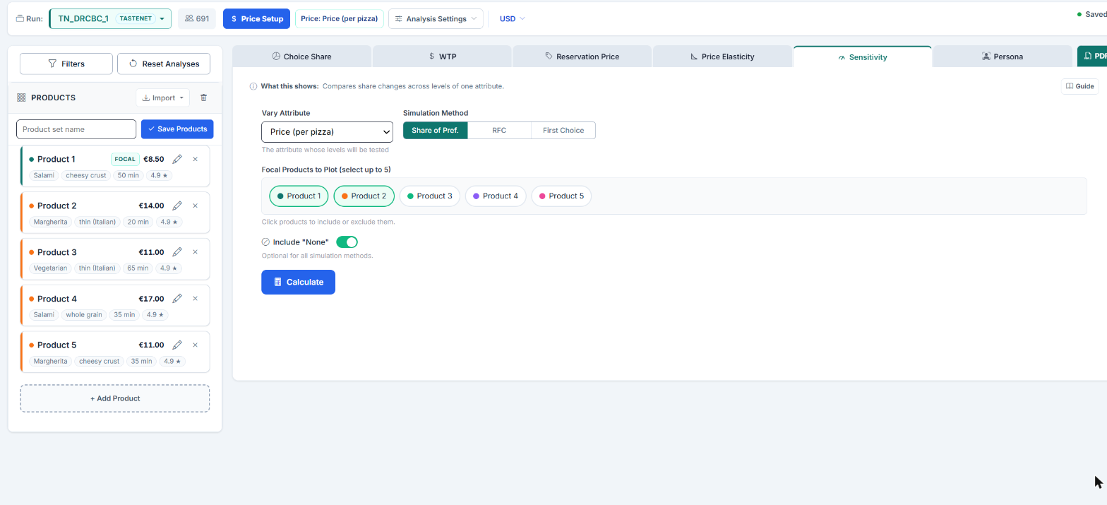
Navigate to the Sensitivity tab. Go to Project, Analysis, Market Simulation, then switch to the Sensitivity tab in the results panel on the right. This is where you configure and run the analysis.
The Sensitivity tab provides the following controls:
The Sensitivity tab reads the products from the Products panel and uses at most the first 10 of them. If you have more, a note above the configuration says how many products you have, that only the first 10 are shown, and that you can select up to 5. With six to ten products the note only states the five-product cap.
Respondent filters are set outside the tab, through the Filters button above the Products panel. Any filter you apply there is sent along with the run and produces an extra result per filter group next to the full sample.
When the varied attribute is the price attribute from Price Setup, respondents who prefer higher prices or barely react to price are left out, as in WTP, Reservation Price and Price Elasticity: their share rises with price and would make the curves climb again at high prices. Include unusual price responses in price analyses in Analysis Settings keeps them. Other attributes always use all respondents, like Choice Share.
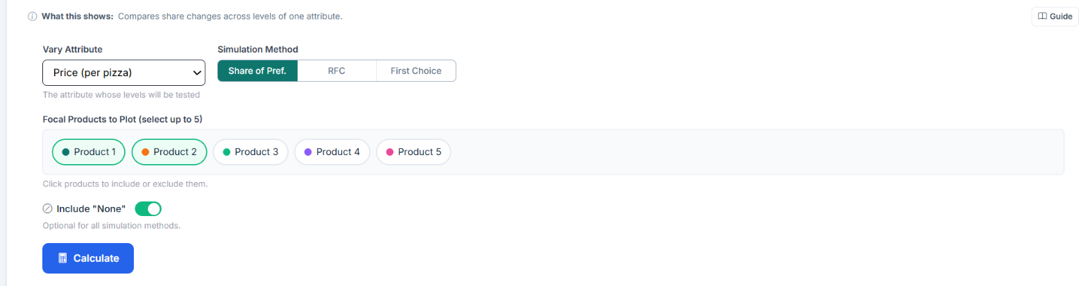
Click Calculate. Choicery iterates through every level of the chosen attribute, swaps it into each focal product one at a time, runs the simulation, and collects the share results. The button shows "Analyzing..." while the run is in progress. The chart, the crossover list and the data table appear once all levels have been evaluated.
If no attribute is selected, or no product pill is active, Choicery refuses to start and says so. The size of a request is the number of plotted products times the number of tested levels times the number of filter groups (at least 1). Above 500 combinations the run is rejected with "Sensitivity combinations is above the synchronous safety threshold (N requested, maximum 500). Reduce the request size."; reduce the number of levels, products or filter groups in that case. RFC runs are also rejected when the requested number of draws exceeds the synchronous cap.
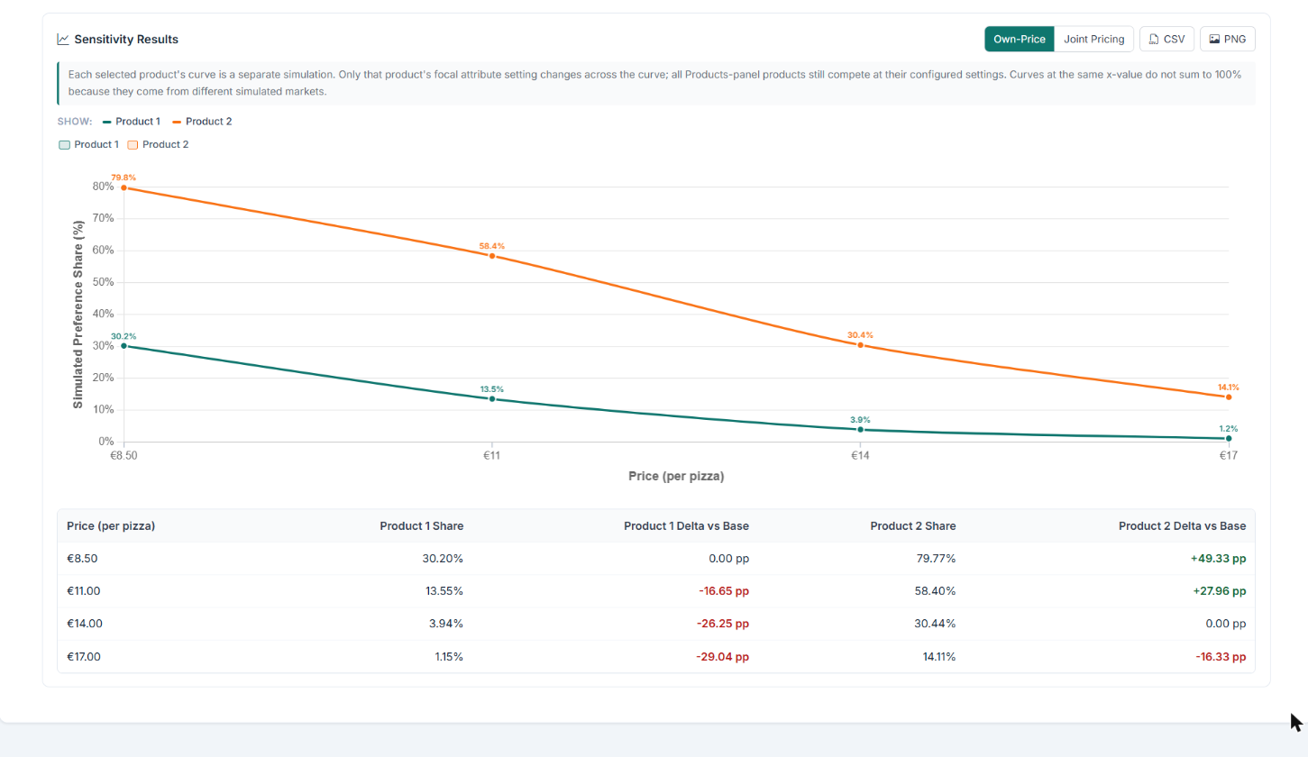
The primary output is a line chart with attribute levels on the X-axis and the simulated preference share (%) on the Y-axis (axis title "Simulated Preference Share (%)"). Each focal product is shown in its own color and every point carries its share as a label. Reading left to right, you can see exactly how share rises or falls as the attribute level changes.
Whether the points are connected depends on how the attribute was estimated. A linear-coded attribute (typically a numeric price) gets a connected, slightly smoothed line, because the values lie on a continuum. A categorical attribute gets markers only, with the share label beside each marker: its level utilities are estimated independently, and a connecting line would suggest a continuum that does not exist.
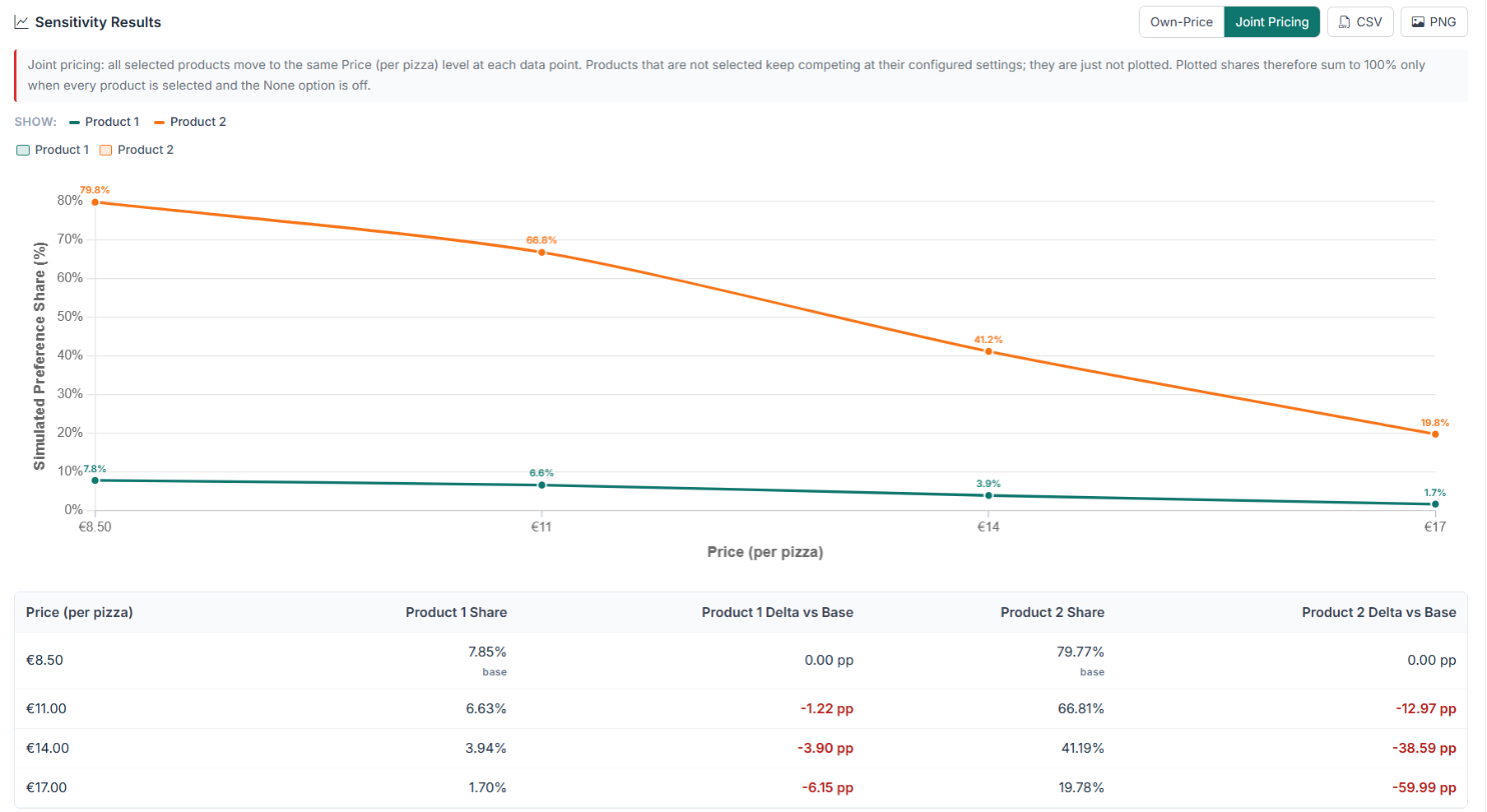
The results header carries a pricing mode toggle with two buttons. Switching it re-runs the analysis immediately.
Above the chart a Show: row appears with filter pills, one group for samples (Overall plus each active filter group) and one group for products, whenever there is more than one of them. These pills only show or hide curves, they do not change the simulation.
A crossover point is where two products' share curves intersect, the level at which the competitive ranking reverses. Choicery detects these automatically for every pair of plotted products and lists them in a Crossover Points block below the chart. The block is hidden when no crossing was found.
Each entry reads "Product A & Product B cross at <level> (share: XX.X%)". When each of the two adjacent
levels has a stored value in the run, or its label contains exactly one unambiguous number (for example
"25000", "EUR 25000.50" or "0,325 €", but not "25,000" or "1.500", which could be a decimal or a
thousands separator), the crossing level is linearly interpolated and printed with a
tilde, for example ~27500. Otherwise the entry names the two levels the crossing falls
between. A note in the same block states that crossover points are linearly interpolated between tested
levels.
Product A leads Product B at the 25000 level (35% vs. 28%) but trails at the 30000 level (24% vs. 31%). The gap is +7 pp at 25000 and -7 pp at 30000, so the crossing lies halfway between the two levels. Choicery interpolates:
Below that point Product A wins. Above it Product B takes the lead.
If you applied respondent filters through the Filters button, an extra block appears under the chart, titled Sensitivity: Overall vs followed by the name of the active group (or "Segments" when several are active). It is a compact table with one row per product and these columns:
Groups that produced no result are listed underneath as errors, for example when no respondent matches the filter. Without active filters this block stays hidden.
The full numeric results are presented in a table below the chart. The first column is named after the varied attribute, and each plotted product contributes two columns, its share and its delta versus base:
| Body Type | Product A Share | Product A Delta vs Base | Product B Share | Product B Delta vs Base |
|---|---|---|---|---|
| Sedan | 28.40% | −6.10 pp | 31.20% | +2.80 pp |
| SUV | 34.50% base | 0.00 pp | 28.40% base | 0.00 pp |
| Hatchback | 22.10% | −12.40 pp | 33.70% | +5.30 pp |
| Wagon | 26.80% | −7.70 pp | 30.50% | +2.10 pp |
Shares and deltas are printed with two decimals. The base badge sits directly below the share of the level that the product is currently configured to in the Products panel; that share is the reference for the deltas, which are expressed in percentage points (pp). In Joint Pricing mode the first tested level serves as the base instead. Positive and negative deltas are colored.
When filters are active the table is split into labeled blocks: first "Overall (full sample)", then one block per filter group with its respondent count.
Two buttons sit in the results header, next to the pricing-mode toggle:
sensitivity_<mode>_<attribute>.csv, for example sensitivity_own_price_price.csv. Its columns are Sample, the attribute, and one share column per plotted product. Filter groups are appended as additional rows in the Sample column.sensitivity_<mode>_<attribute>.png.The PDF button in the tab bar produces a "Sensitivity Analysis" report from the currently displayed result.

When you select the price attribute as the varied attribute, the resulting chart is a demand curve: price on the X-axis, market share on the Y-axis. This is one of the most valuable outputs of conjoint-based market simulation. Keep in mind that the X-axis carries the price levels of your design, in design order, and that the points are connected into a line only if price was estimated as a linear attribute.
An important subtlety: even when using a main-effects HB model (no explicit interaction terms), the simulation reveals brand-by-price interactions implicitly. This happens because each respondent has individual-level utilities, and the logit share calculation is nonlinear. As Orme (2020, Ch. 17) notes, this is one of the key advantages of individual-level HB estimation over aggregate models.
The methodology behind sensitivity analysis in conjoint-based market simulation.
The sensitivity analysis algorithm proceeds as follows:
Define the base case. Record the current level of every attribute for every product in the simulation. This is the starting point.
Determine the base share. Each focal product's base share is its simulated share at the level it currently has in the Products panel. Choicery reads it from the same sweep as the other levels and simulates the configured level additionally if it is not among the tested levels. In Joint Pricing mode the first tested level is the base.
Iterate through levels. For each level l of the chosen attribute:
Compute deltas. For each level, calculate the difference from the base share: Delta = Share(level l) − Share(base)
Step 3 is where the two pricing modes differ. In Own-Price mode the loop runs once per focal product, so product j's curve comes from simulations in which only product j moved. In Joint Pricing mode there is a single loop over levels in which all focal products are set to level l simultaneously, so one simulation per level feeds all curves at once. Non-focal products keep their base configuration in both modes.
The per-product summary statistic Choicery reports is the share range, the plain difference between the highest and the lowest simulated share across the tested levels:
Consider a TV conjoint with attributes: Brand, Screen Size, Sound, and Price. A Sony TV has base share of 33%. Sensitivity on key attribute changes reveals:
The results immediately highlight that dropping surround sound would be devastating (−20 pp), while adding channel blockout provides the largest positive lift (+15 pp). This kind of product-specific, competitively-contextualized insight is what makes sensitivity analysis invaluable for product design decisions.
When two products' share curves cross between adjacent tested levels, Choicery estimates the exact crossover using linear interpolation:
This formula finds the point where the share difference between Product A and Product B passes through zero, assuming a linear relationship between the two tested levels.
| Attribute Type | Crossover Reporting | Example |
|---|---|---|
| Numeric labels (e.g., Price) | Both adjacent levels have a stored value or a label with exactly one unambiguous number, so the value is interpolated and printed with a tilde | "Product A & Product B cross at ~28000" |
| Non-numeric labels (e.g., Body Type) | No value can be interpolated, so the two bracketing levels are named | "Product A & Product B cross at between Sedan and SUV" |
Attribute importance scores (derived from the range of part-worth utilities) are a useful summary of how much each attribute could matter. But they have significant limitations that sensitivity analysis overcomes:
| Dimension | Raw Importance Scores | Sensitivity Analysis |
|---|---|---|
| Scope | Attribute-level (averaged across all products) | Product-specific (accounts for each product's position) |
| Competitive context | None, ignores what competitors offer | Full, all products compete simultaneously |
| Interaction effects | Not captured (attribute-level aggregation) | Implicitly captured via individual-level HB utilities in nonlinear logit simulation |
| Output metric | Abstract percentage (0 to 100% importance) | Actionable share percentages and pp deltas |
| Decision support | "Price is the most important attribute" | "Dropping price from €30k to €25k gains 8 pp share against Product B" |
The key insight is that importance scores are context-free while sensitivity results are context-dependent. The same attribute may have high importance but low sensitivity if all products in the market already offer similar levels. Conversely, a low-importance attribute can produce large share swings if it is the key differentiator between two closely matched products.
Orme, B. K. (2020). Getting started with conjoint analysis: Strategies for product design and pricing research (4th ed.). Manhattan Beach, CA: Research Publishers LLC.
Orme, B. K., & Chrzan, K. (2017). Becoming an expert in conjoint analysis: Choice modeling for pros. Orem, UT: Commercial conjoint software publisher