How to simulate competitive markets and predict product shares using conjoint utilities, a practical guide for Choicery with methodological background.
Everything you need to set up, run, and interpret market simulations in Choicery.
Market simulation takes the individual-level utilities from your HB (or TasteNet) estimation and places product concepts in simulated competition. You define products with specific attribute levels, and the simulator predicts how respondents would distribute their choices among those products.
Think of it this way: imagine all your survey respondents gathered in one room, presented with a shelf of products, and each one picks their favorite. The simulator does this computationally, using each respondent’s estimated preferences to determine their choice.
Choice shares (%) for each product, the predicted proportion of respondents who would choose each product in the defined competitive scenario. If Product A gets 35% and Product B gets 65%, the model predicts that 35% of respondents would prefer Product A when faced with that specific choice.
This is the most practically important feature in conjoint analysis. While HB estimation tells you what people prefer in general, market simulation answers the “What if?” questions that drive business decisions:
HB estimation is the engine: it extracts individual preferences from choice data. Market simulation is the steering wheel: it lets you explore any competitive scenario using those preferences. You run estimation once; you run simulations many times.
Before running a market simulation in Choicery, you need the following:
The Guide button at the top right of the Choice Share tab opens this tutorial: that is the in-app entry point for users who want to read the background while configuring a simulation.
A completed analysis run with individual-level utilities. The simulator uses each respondent’s individual part-worth utilities as input. Without these, there is nothing to simulate. Run a Preference Analysis (HB) or an AI-Driven Profile Analysis first, from the Analysis page.
Open Market Simulation. On the Analysis page, open the Market Simulation section and click Go to Market Simulation. The simulator opens on its own page with the Products panel on the left and a tabbed results panel on the right. The first tab is Choice Share.
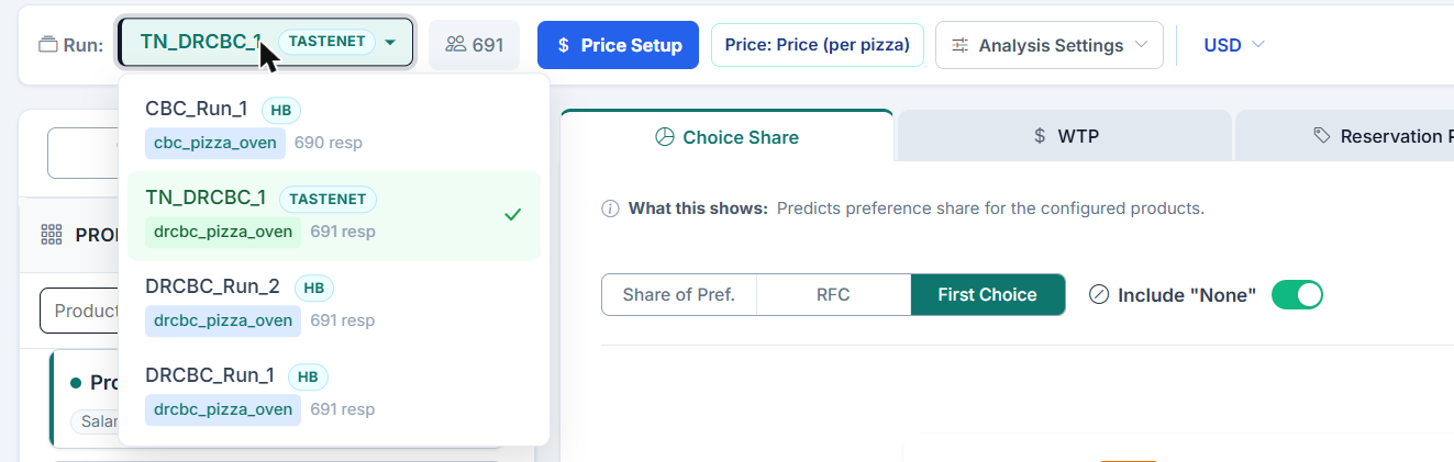
Select the run. The Run: dropdown in the top bar lists every completed run across all conjoint tasks in the project, with the task name and the respondent count. Every run carries a source badge, HB or TasteNet, both in the list and on the selected run. All simulator tabs use the run selected here.
Configure Price Setup (if applicable). If your study includes a price attribute and you plan to use the WTP, Reservation Price, or Price Elasticity tabs, click Price Setup in the top bar first. This tells the simulator which attribute represents price and what the numeric values of its levels are. Choice Share itself does not require it.
With no completed run the controls are disabled and the tab shows Choice Share Not Available with the note “No completed analysis run found. Select a conjoint task and run a Preference Analysis (HB) or AI-Driven Profile Analysis before using Market Simulation.” Run an estimation from the Analysis page first, then return here.
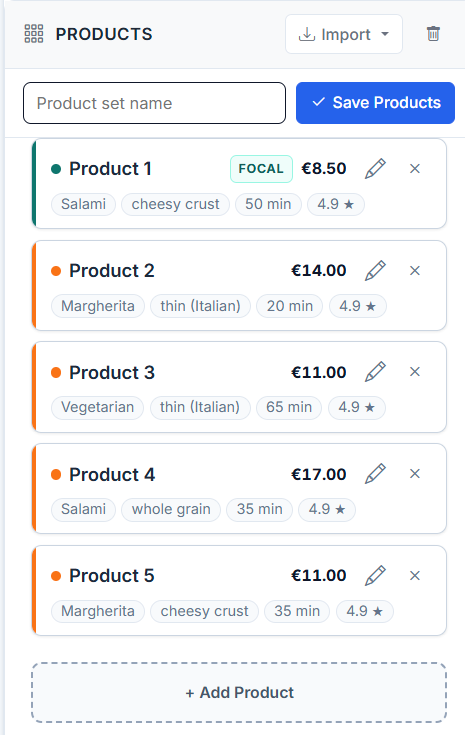
The Products panel (left side of the simulator) is where you define the competitive scenario. Each product is a hypothetical offering defined by selecting one level for each attribute in your conjoint study. The same product set feeds all simulator tabs, not just Choice Share.
Each product appears as a card with an editable name field, an Edit (pencil) button that expands the attribute controls, a Remove (x) button, and one control per attribute. Categorical attributes get a dropdown of their levels, linear attributes get a free numeric input. The first card carries a Focal badge, marking it as the default focal product. Reservation Price always analyses that first product (its caption reads “Calculating reservation price for <name> from the Products panel”), while the WTP and Price Elasticity tabs have their own Focal Product dropdown, and Sensitivity lets you pick up to five products to plot. For example, a car study might have:
For the most actionable insights, define products that represent actual market offerings. Include your own product and your key competitors with their real attribute levels. Then modify your product to test “what if” scenarios.
Choicery offers three methods for computing choice shares from individual-level utilities. Choosing the right method is the most important decision in simulation setup. Each method makes different trade-offs between precision, robustness to competitive structure, and interpretability.
The method is picked with the three-way selector at the top of the Choice Share tab. The options are labelled Share of Pref., RFC and First Choice, in that order. Share of Pref. is preselected. Hovering an option shows a one-line description of the method.
RFC is worth considering when the product set contains very similar competing products: it addresses IIA limitations via similarity-corrected Monte Carlo. It was proposed by Bryan Orme (1998) specifically to address limitations of the other two methods.
For each respondent, the simulator runs many simulated “shopping trips” (default: 1,000 iterations). In each trip:
The product’s share for that respondent is the fraction of shopping trips in which it was chosen. Shares are then averaged across all respondents.
When two products share attribute levels (e.g., both are Brand A, both have a 5-year warranty), the random shocks on those shared levels are identical. This means near-identical products get highly correlated noise, causing them to compete primarily with each other, not with dissimilar products. This elegantly solves the IIA problem (see Section 13).
Selecting RFC reveals an Advanced Settings toggle below the method selector. Expanding it shows five fields:

Share of Preference computes each respondent’s choice probability via the softmax function (the multinomial logit rule):
Each respondent “splits” their vote probabilistically across all products. A respondent with utilities of 5.0, 3.0, and 2.0 for three products doesn’t just vote for product 1: they give it a high probability (about 73%) while still allocating some probability to the other products.
First Choice is the simplest method: each respondent votes for the single product with the highest total utility. No probabilities, no noise, just a straight vote.
The following table summarizes when each method is most appropriate:
| Scenario | Best Method | Why |
|---|---|---|
| General purpose with HB-estimated data | Share of Preference (UI default) | Deterministic, no Monte Carlo variance, recommended for HB |
| Many similar / clone products | RFC or First Choice | Similarity correction reduces IIA; First Choice nearly eliminates it |
| Need deterministic, reproducible results | Share of Preference | No Monte Carlo variance, identical results every run |
| Small sample, need maximum precision | Share of Preference | Probabilistic voting extracts more info per respondent |
| Strict "each respondent picks max-utility product" | First Choice | Fast, deterministic, no probability spreading; "each person picks their favorite" is intuitive |
| Calibrating toward observed market shares | RFC, calibrated on holdouts | The simulator has no scale-factor field; the RFC variability parameters are the tunable settings (see Section 10.3) |
Share of Preference is the UI default and the recommended method for HB-estimated data: it is fully deterministic (no Monte Carlo variance) and HB already substantially reduces IIA. Switch to RFC if your product set contains very similar competing products and you want the explicit similarity correction. Use First Choice when you want the strictest "each respondent picks their max-utility product" rule (fast, deterministic, no probability spreading).
The Include “None” toggle, next to the method selector, adds a no-purchase alternative to the simulation. This represents respondents who would not buy any of the defined products. It is on by default.
The None option is only available if the estimation behind the selected run included a None option (i.e., the conjoint design had a “none of these” alternative and a None utility was estimated). If it was not, the control area shows the note “None not available in active run”.
| Setting | Interpretation | Shares Sum To |
|---|---|---|
| None OFF | Forced choice: every respondent must pick one of the defined products | 100% (among defined products) |
| None ON | Respondents can opt out; None share = “would not buy any” | Product shares + None share = 100% |
The None share is relative to the specific products in the scenario. Adding a very attractive product will reduce the None share; removing products will increase it. Do not interpret the None share as an absolute measure of market demand: it depends entirely on the defined competitive set.
Click Run Simulation after defining your products and selecting a method. Results appear immediately for Share of Preference and First Choice, or after a moment for RFC with many iterations.
Each alternative gets a share card with its choice share as a percentage. The cards follow the order of the Products panel as it was when the simulation ran, with None last. The product with the highest share among the products carries a Winner tag; None never does, and no tag is shown when two products tie at one decimal place. Below the cards, a horizontal bar list shows the same shares sorted from largest to smallest, and a line above the cards states the None share in words when it is included.
A meta line under the bars records how the numbers were produced: the method, and for RFC the iteration count, the variability settings and the seed actually used, plus +None when the None option was included and the segment sample size when a filter is active. Quote that line whenever you report a share, because RFC numbers are only reproducible together with their seed.
Interpretation: In this three-way competition, Brand A captures the largest share, likely due to its favorable price-feature combination. Brand C trails, possibly penalized by its higher price.
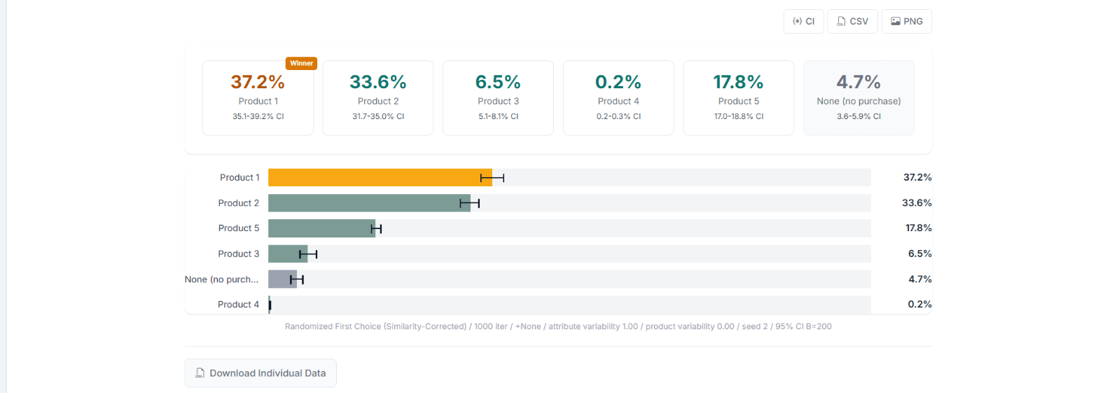
The CI button above the results computes 95% percentile confidence intervals for the shares by resampling respondents with replacement (200 bootstrap draws, seed 1). The interval is then printed on each share card and drawn as a marker on the bar, the meta line adds “95% CI B=200”, and the CI method, level, number of bootstrap draws and bootstrap seed are added to the CSV export. Use it before claiming that one product beats another: if the intervals overlap heavily, the ranking is not established by your sample.
Two export buttons sit in the results header, next to CI, and a third below the result block:
choice_share.csv: a header block with the method and its parameters, the aggregate shares (with standard deviations and confidence intervals where available), and the per-respondent rows.individual_data.csv with one row per respondent. For First Choice it contains the chosen product and the utility of every product; for Share of Preference and RFC it contains each respondent’s probability per product.The individual file is useful for identifying respondent clusters, linking choices to survey demographics, or spotting unusual preference patterns. It is a download only: there is no inline per-respondent table in the tab.
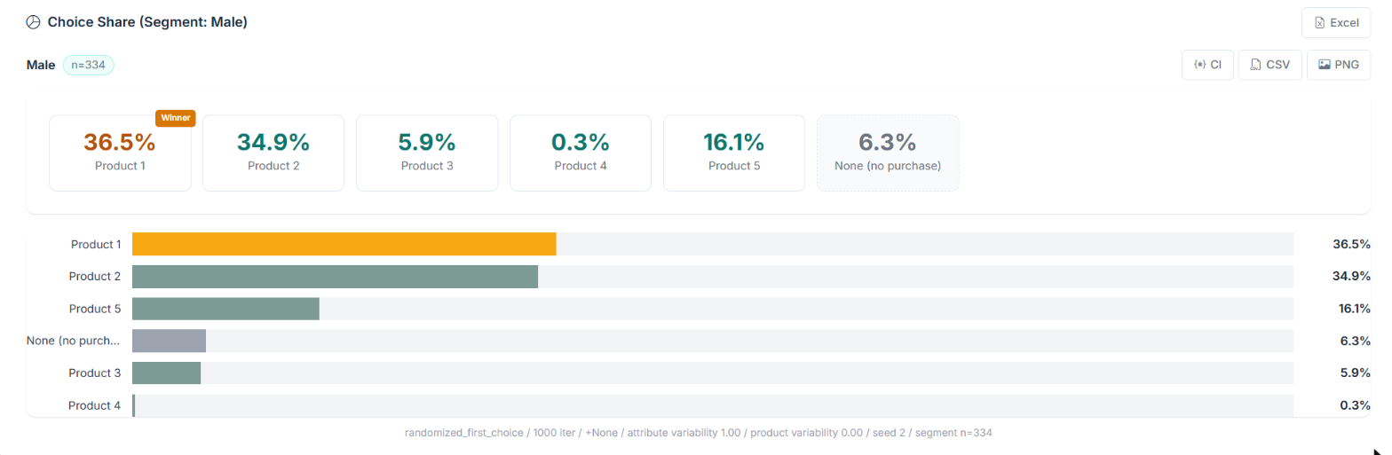
When filters are active (see Section 7), a second block appears below the main results with one sub-block per segment, each with its own share cards, bars, respondent count (n=...) and its own CSV / PNG buttons; the CI button appears once the segment result is stored and the segment has at least two respondents. The heading reads Choice Share (Segment: <name>) when exactly one filter is active, and Choice Share (Segments) when there are several. This answers: “Do different demographic or attitudinal groups prefer different products?”
Younger respondents prefer Product A more strongly, while older respondents lean toward Product B. Product C is relatively stable across age groups.
The PDF button at the right of the simulator tab bar exports the currently open tab. From Choice Share it produces the Choice Share Simulation report, containing the settings used, the active filters, the aggregate shares and, when present, the per-segment results. The export uses the results currently on screen, so run the simulation before requesting the PDF.
A product set is the current product configuration stored under a name. This is how you keep “what-if” configurations side by side:
Use descriptive names: “Baseline: Current Market”, “Price Increase +10%”, “New Competitor Enters”. This makes it easy to recall what each set represents when you return later. Product sets store the products only. The method, the None toggle and the RFC settings are not part of a set; they stay as currently set in the Choice Share tab and are remembered per user between visits.
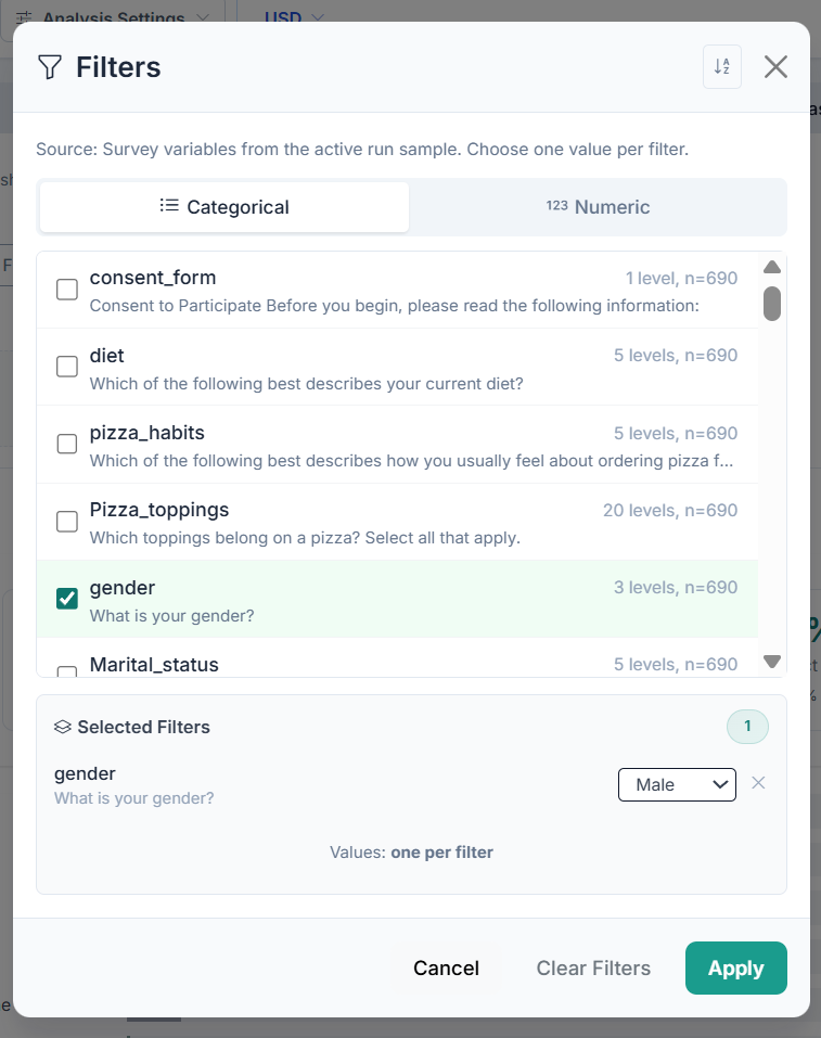
The Filters button above the Products panel restricts the simulation to a subgroup of respondents based on their survey responses. The modal has a Categorical and a Numeric tab, and the variables offered are the survey variables of the active run sample (for AI-Driven Profile Analysis runs the Categorical tab offers the run’s profile groups instead):
Selected filters are listed in the modal; Apply activates them, Clear Filters removes them. When filters are active, the simulation is computed both for the full sample and for each filtered subgroup, so the overall result and the segment results stay comparable.
Filters work on the same people as the overall result: everyone in the selected estimation run. The answers come from the current data, so a value corrected in the Data Editor counts in its new group. A response moved to the bin after the run is still part of the run and therefore still counts in its segment; to leave it out of both, estimate the model again. Responses collected after the run are not part of it and appear in no segment.
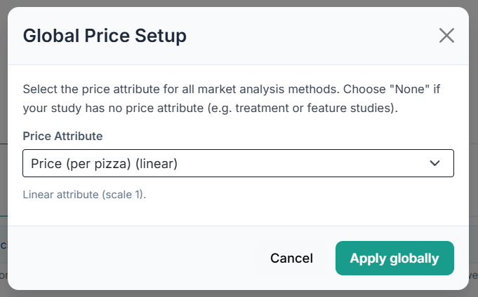
Price Setup in the top bar opens the Global Price Setup dialog. It tells every market analysis method which attribute represents price, and for categorical price attributes what each level is worth numerically. Click Apply globally to store the choice. It is required for:
For categorical price attributes, you enter a numeric value per level (e.g., “Budget” = 19.99, “Standard” = 29.99, “Premium” = 49.99). For linear price, no mapping is needed since the levels are already numeric. If your study has no price attribute at all (a treatment or feature study), select the “(None - no price attribute)” entry and the price-based methods stay disabled.
The money amounts are shown in the currency selected in the top bar next to Price Setup; the selector also controls whether the symbol is printed before or after the number.
Analysis Settings, next to Price Setup, holds three shared toggles for the price-based tabs: Include unusual price responses in price analyses (keep respondents with a positive or near-zero price response), Exclude outliers (drop outliers before aggregation), and Allow negative prices. They apply to WTP, Reservation Price, Price Elasticity and the Sensitivity tab when it sweeps price. Choice Share always uses all respondents.
Presenting simulated shares to management as if they were real market shares. Simulated shares predict preference, not purchasing behavior. Always caveat that shares do not account for availability, awareness, habit, or switching costs.
Mathematical foundations, the IIA problem, and the algorithms behind the three simulation methods.
The Share of Preference method applies the multinomial logit (softmax) function to each respondent’s utilities:
The aggregate share for product j is the average across all N respondents:
Where Vij is the total utility of product j for respondent i, computed as the sum of part-worth utilities for the product’s attribute levels.
CBC utilities estimated by HB tend to be too large in magnitude compared to real-world choice behavior. This produces simulated shares that are too extreme: the best product gets a share of, say, 85% when its real market share might be 35%.
A scale factor λ < 1 can be applied to flatten shares toward reality. Louviere (1988) suggests values around 0.3 to 0.5 depending on the study. With λ = 1.0, the raw HB utilities are used as-is.
The Choice Share tab does not expose a scale factor: Share of Preference always runs at λ = 1.0 on the raw individual utilities. The example below is there to explain what a scale factor does and why raw logit shares look extreme, not to describe a setting you can change. If you need flatter, calibrated shares, use RFC and tune its variability parameters against holdout choices.
As λ decreases, shares move toward equal (1/J). The “right” scale factor is the one that best calibrates to known market data.
The logit model has a well-known structural limitation: the Independence of Irrelevant Alternatives (IIA). This is covered in full detail in Section 13, but the key implication for Share of Preference is this: adding a product that is nearly identical to an existing one will draw share from all products proportionally, not just from the similar one. This can produce seriously misleading results when the competitive set includes similar products.
If you add a clone of Product A to the simulation and use Share of Preference, both Product A and its clone will each get about half of what Product A had before, but so will Products B and C, losing share proportionally. In reality, the clone should primarily cannibalize Product A while leaving B and C nearly unaffected.
Each respondent votes for the single product with the highest total utility:
The standard error of each share estimate follows the binomial proportion formula:
This is the textbook standard error of a proportion. Choicery does not print it; the CI button uses a respondent bootstrap for all three methods (Section 6.3).
RFC was proposed by Bryan Orme in 1998 to combine the strengths of First Choice (IIA resistance) with those of Share of Preference (precision), while adding a similarity correction mechanism. It is widely used in conjoint analysis when product sets contain near-substitute alternatives.
RFC is a Monte Carlo method. For each respondent, the algorithm runs M simulated “shopping trips” (Choicery starts at M = 1,000):
The critical detail is in how noise is applied: for an attribute using similarity correction, the random shock is drawn once per attribute level, not once per product. Every product that shares that level receives the exact same shock. Price is uncorrelated by default because correlated price error can create artificial kinks in demand curves; it can be enabled explicitly for a justified design.
Consider three products in a car study:
In one shopping trip, suppose the simulator draws:
Then the noise added to each product is:
Products A and B share “Brand A” (+0.8 for both). Products A and C share “Hybrid” (+0.5) and “5yr warranty” (+0.3). This creates correlated fluctuations between similar products, making them substitute from each other in realistic patterns.
The key insight is that products sharing many attribute levels have highly correlated noise. If two products share 4 out of 5 attributes, 80% of their random shocks are identical. When one gets a positive shock, the other does too. This means:
RFC generalizes both other methods as limiting cases:
| Condition | RFC Reduces To |
|---|---|
| σa = 0 for all attributes (no noise) | First Choice, the argmax of the raw utilities is always chosen |
| Attribute variability 0, product variability 1 (a unit Gumbel error per product, no attribute-level noise) | Share of Preference (Logit) at scale factor 1; other product variabilities correspond to other scale factors |
In Choicery, the RFC defaults are:
Iterations, attribute variability and product variability are also bounded server-side: iterations must stay within the accepted range, and both variability parameters within 0 to 5.
Some conjoint simulators determine variability and iteration settings automatically. Choicery exposes explicit custom parameters instead. Use holdout choices or observed choices to calibrate them before treating absolute simulated shares as forecasts.
The CSV export carries each product’s standard deviation across iterations (column Std (%)); it is not shown on the cards. If this value is large relative to the share differences between products, increase the number of iterations. At 1,000 iterations the Monte Carlo error of a share is about one share point; increase iterations when the products you want to rank are closer than that. Choicery additionally checks whether adjacent products in the ranking are separated at the 95% Monte Carlo level; if they are not, the meta line under the results says “MC precision: adjacent ranking overlaps”, which means the ranking of those two products is not resolved by the number of iterations you ran.
The Independence of Irrelevant Alternatives (IIA) is the single most important theoretical issue in market simulation. Understanding it is essential for choosing the right simulation method and interpreting results correctly.
A choice model satisfies IIA if, for any two alternatives A and B:
This is a direct consequence of the logit model’s mathematical structure (McFadden, 1974). In the softmax function, each product’s probability depends only on its own utility relative to the sum of all utilities: there is no notion of “similarity” between products.
This is the classic illustration of IIA, originally described by McFadden (1974):
Consider a city where commuters choose between a car and a red bus. Suppose the shares are:
Now the city introduces a blue bus that is identical to the red bus in every way (same route, same schedule, same price) except for its color. What should happen?
Intuitively correct answer: The blue bus should split the bus riders, not the car riders:
Logit (IIA) answer: The logit model treats the blue bus as an independent alternative. Since P(Car)/P(Red Bus) must remain constant at 50/50 = 1:
The logit model wrongly predicts that the blue bus steals equally from the car and the red bus. In reality, a commuter who prefers buses would choose between the two buses; a commuter who prefers driving would be unaffected by the bus color.
A more practical illustration relevant to conjoint research:
Suppose a beverage study finds these initial shares:
Now we add Coke Zero to the simulation. Coke and Coke Zero share the brand, the packaging, the distribution: they are near-substitutes that differ mainly on calories.
Realistic expectation: Coke Zero primarily cannibalizes Coke. Pepsi loses a little (some Pepsi drinkers might switch). Milk is unaffected.
Share of Preference (IIA) outcome: All existing products lose share proportionally:
Under IIA, Milk loses over 6 share points to Coke Zero, despite the two products having nothing in common. This is clearly unrealistic.
IIA produces the most misleading results when the competitive set includes products that are close substitutes for each other but not for all products. If all products are equally (dis)similar, IIA is less of an issue. The more lopsided the similarity structure, the more IIA distorts results.
With aggregate-level (pooled) utilities, every respondent has the same preferences, and IIA is at its worst. HB (Hierarchical Bayes) individual-level utilities substantially reduce the IIA problem (Orme, 2020).
Here is why: different respondents have different preference patterns. Some are brand-loyal (Coke lovers who would never drink Pepsi), others are price-sensitive (switching at any price difference), and others have unique idiosyncratic preferences. When you average across these heterogeneous individual choices, the aggregate substitution patterns become more realistic.
Consider adding Coke Zero with individual-level utilities:
Because each respondent’s substitution is driven by their own preferences, the aggregate result naturally reflects realistic competitive dynamics. Coke loses the most to Coke Zero, Pepsi loses little, and Milk loses only to the extent that some health-conscious respondents are attracted by the zero-calorie option.
However, HB does not fully eliminate IIA. Within each respondent’s logit model, the IIA property still holds. The correction comes from aggregating across heterogeneous respondents, not from fixing the model at the individual level.
RFC adds an additional layer of IIA correction on top of HB’s individual-level heterogeneity. The attribute-level correlated shocks create explicit similarity-based substitution:
The combination of HB heterogeneity + RFC similarity correction provides the strongest defense against IIA in practical conjoint simulation.
Simulated choice shares should never be equated with actual market shares. They represent preference shares, the share of stated preferences among the defined products, given the attributes measured in the conjoint study.
To convert preference shares to approximate market share predictions, you would need to account for many factors not captured in the conjoint model:
Simulation shares are excellent for relative comparisons: “Product A would have about 1.5x the share of Product B,” or “Raising the price by 10% would cost us about 5 share points.” The direction and relative magnitude of share changes are typically reliable even when the absolute numbers are not.
One of the most actionable analyses you can perform is a Source of Volume (or “switchback”) analysis:
Product X draws most of its share from Competitor A, suggesting they are the closest substitute. This information is invaluable for positioning and competitive strategy.
Systematically varying one attribute level while holding all others constant produces a demand curve (or “sensitivity plot”) for that attribute. For price, this is a classic price-response curve:
The same approach works for any attribute: vary the feature level and observe how share responds. This reveals which attribute improvements have the greatest impact on market position.
You do not have to do this by hand. The simulator carries a Sensitivity tab that sweeps an attribute automatically against the products you defined, and a Price Elasticity tab that produces the price-response curve and the elasticity for a focal product. Both have their own methodology guides, reachable from the Guide button on those tabs.
Running the same scenario with all three methods serves as a robustness check:
Luce, R. D. (1959). Individual choice behavior: A theoretical analysis. New York: Wiley.
McFadden, D. (1974). Conditional logit analysis of qualitative choice behavior. In P. Zarembka (Ed.), Frontiers in econometrics (pp. 105-142). New York: Academic Press.
Orme, B. K. (1998). Randomized first choice. Conjoint Analysis Research Paper Series.
Orme, B. K. (2020). Getting started with conjoint analysis (4th ed.). Manhattan Beach, CA: Research Publishers LLC.
Orme, B. K., & Chrzan, K. (2017). Becoming an Expert in Conjoint Analysis.
Rao, V. R. (2014). Applied conjoint analysis. New York: Springer.
Train, K. E. (2009). Discrete choice methods with simulation (2nd ed.). Cambridge: Cambridge University Press.