How to detect and interpret attribute interaction effects in conjoint data. Every setting of the form, how to read the results, and the method behind it, with the pizza oven CBC of the Pizza (Example) study as worked example.
Everything you need to run, interpret, and export Interaction Search analyses in Choicery.
1. What Are Interaction Effects?
Interaction effects occur when a consumer’s preference for one attribute depends on the level of another attribute. In a standard conjoint model, we assume that preferences are additive, the utility contribution of each attribute level is independent of every other attribute. Interaction Search tests whether this assumption holds.
The core idea
Consumers might love red for an SUV but hate red for a sedan, the effect of color depends on body type. If such a pattern exists in your data, the additive main-effects model is missing something. Interaction Search finds these patterns.
Standard conjoint models estimate main effects only: each attribute level gets a single utility weight that applies regardless of what levels appear on the other attributes. This additive structure keeps the model simple and interpretable. But sometimes, certain attribute combinations create value (or destroy it) beyond what the individual main effects predict.
Example: Brand × Price
Suppose a conjoint study has three brands (A, B, C) and three price levels ($10, $20, $30). Under the main-effects model:
U(Brand A, $10) = U(Brand A) + U($10)
U(Brand A, $30) = U(Brand A) + U($30)
But what if Brand A is a luxury brand? Consumers might actually prefer the higher price for Brand A (signaling quality) while strongly penalizing the same price for Brand C (a budget brand). In that case, Brand × Price has an interaction effect, the price sensitivity differs by brand.
In Choicery, Interaction Search runs a likelihood-ratio chi-square test on every pair of attributes to detect significant interactions. It compares a main-effects-only model against a model that includes cross-product terms for each attribute pair, one pair at a time.
Analogy
Think of it as testing whether 1 + 1 really equals 2 for each attribute combination, or whether certain combinations create something more (or less) than the sum of their parts.
2. Prerequisites
Before running Interaction Search in Choicery, make sure you have the following:
1
A conjoint task with at least 2 attributes. Interaction Search tests pairs of attributes, you need at least two to form a pair. Supported conjoint types: CBC, CBC Shop, DR-CBC, and BW-CBC.
2
Collected survey responses, at least ~100 respondents recommended. Interaction Search uses an aggregate MNL model. Technically the run only aborts below 5 valid choice observations, but with fewer than 100 respondents the model may not converge reliably and p-values may be unreliable. More data (200+) gives more statistical power to detect genuine interactions.
3
Navigate to Conjoint Analysis → Interaction Effects tab. From your project, go to Analysis → Conjoint Analysis. At the top of the page you will see four analysis-type tabs: Preference Analysis (HB), AI-Driven Profile Analysis, Latent Class, and Interaction Effects. Click Interaction Effects. The tab is disabled for tasks it does not support (MaxDiff and Anchored MaxDiff), where it carries the tooltip “Conjoint only”.
4
Work through the three workflow steps. Below the tabs, the workflow bar shows 1 Estimation, 2 Results, and 3 Export. Steps 2 and 3 stay disabled until a run has completed. The funnel icon on the left of the same bar opens the Participant Filter; the Methodology Guide button on the right opens this document.
Number of pairs grows quickly
With k attributes, the number of pairs tested is k(k − 1) / 2. For 4 attributes that is 6 pairs; for 8 attributes it is 28 pairs. More pairs means more multiple-comparison corrections and potentially longer run times.
3. Running Interaction Search in Choicery
3.1 Creating a Run
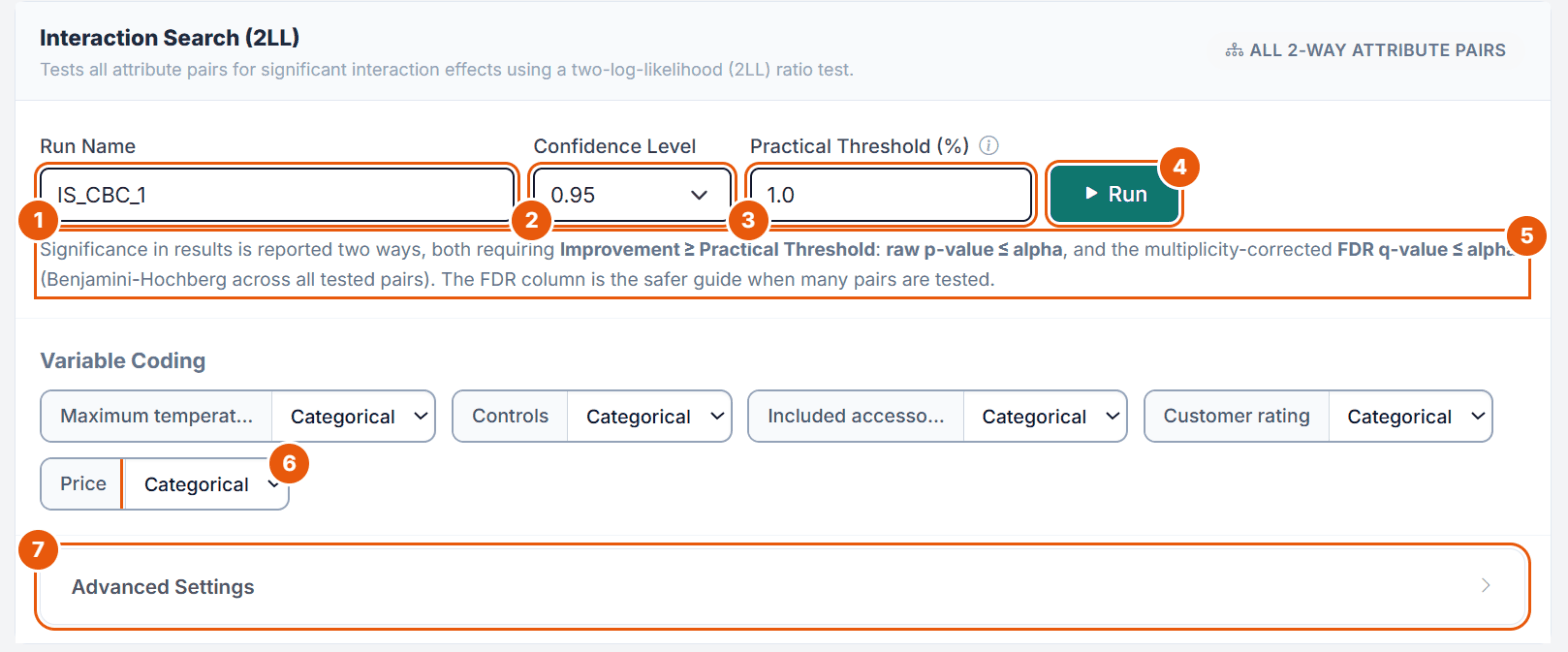
Step 1 Estimation shows a run selector at the top (or an empty-state card reading No Interaction Search Run Yet with the participant count, if this task has no run yet), followed by the estimation card titled Interaction Search (2LL). Figure 1 shows it for the pizza oven CBC (cbc_pizza_oven, 690 respondents) with the default settings.
Figure 1. The Interaction Search form of the Pizza task cbc_pizza_oven.
No.
Control
What it does
1
Run Name
Suggested and counted up per task: IS_CBC_ for CBC, IS_SCBC_ for CBC Shop, IS_Run_ for the other types. Up to 50 characters, unique within the project.
2
Confidence Level
0.90, 0.95 (default) or 0.99. Sets alpha for the significance decisions: 0.10, 0.05 or 0.01.
3
Practical Threshold (%)
Minimum gain in percent certainty, in percentage points, that a pair needs in addition to significance (default 1.0). Section 4.4 shows why this value matters.
4
Run
Starts the analysis (section 3.5).
5
Significance hint
States how results are flagged: raw p-value ≤ alpha and FDR q-value ≤ alpha, both together with Improvement ≥ Practical Threshold.
6
Variable Coding
Categorical or Linear per attribute (section 3.2). The Pizza runs keep every attribute categorical.
7
Advanced Settings
Solver settings of the MNL estimation (section 3.4).
Once a run has completed, its fields are shown read-only. Use New Run (in the run dropdown or the button on the right of the run bar) to unlock the form again; it keeps the settings of the run you were looking at. The trash icon next to a run deletes it. A task can hold at most 10 completed runs; delete an old run to create another.
The practical threshold
Statistical significance alone is not enough. With large samples, even tiny effects become “significant.” The practical threshold ensures that flagged interactions are both statistically reliable and large enough to matter. The default of 1.0 percentage points is strict: in the Pizza study the one interaction with a clear level pattern gains 0.36 points and is not flagged at 1.0 (section 4.4). Lower the threshold, for example to 0.25, when you want to see interactions that matter for specific product combinations rather than for overall fit.
3.2 Variable Coding
Below the run fields, the Variable Coding section lists every attribute of the task with a dropdown offering two options, Categorical and Linear. Choosing Linear reveals one numeric input per level, where you enter the raw value that level represents. Internally the values are centered and scaled by their standard deviation, so effects involving a linear attribute are reported per standardized unit (see the Units chip in the explorer). The run refuses to start if a linear attribute has an empty or non-numeric level value.
Coding
When to Use
What It Does
Categorical (default)
Most attributes (brand, color, features)
Effects-coded, one utility per level, sum-to-zero constraint. This is the standard approach.
A single linear coefficient per attribute. You enter the raw numeric value of each level; internally the values are centered and scaled by their standard deviation, so slope deltas and the linear × linear coefficient are expressed per standardized unit. Reduces the number of interaction parameters.
How coding affects interaction terms
For a categorical attribute with 4 levels and another with 3 levels, the interaction requires (4 − 1) × (3 − 1) = 6 additional parameters. If one is coded as linear, the interaction requires only (4 − 1) × 1 = 3 parameters. Linear coding can be beneficial when you have many levels and want to keep the model parsimonious.
3.3 None Option
An Include None Option checkbox appears only for the task types where the no-choice answer is a separate follow-up question: DR-CBC always, and BW-CBC when the design has a none option. It is pre-checked in those cases. For CBC and CBC Shop the checkbox is not shown; if the design contains a none option, it is included automatically.
The tooltip on the checkbox describes what is included: for DR-CBC a “No” follow-up is treated as None, for BW-CBC a “No” answer after the Best choice is treated as None. Unchecking it estimates from the product-choice stage only.
For BW-CBC only the Best choices (plus the None follow-up when included) enter the model; Worst choices are not modeled by Interaction Search. The results view and the Managerial Summary sheet state this.
3.4 Advanced Settings (Collapsible)
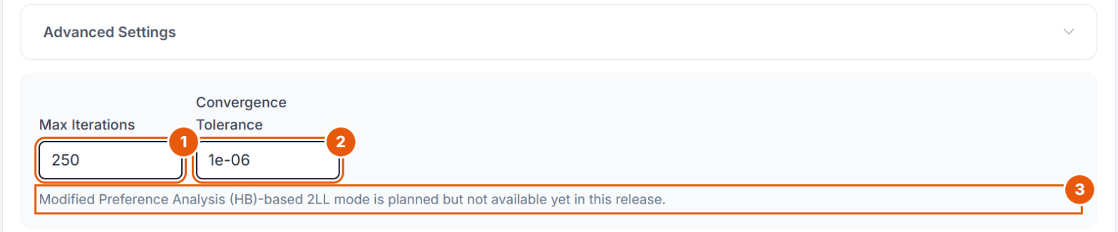
Figure 2. Advanced Settings with their defaults.
No.
Field
What it does
1
Max Iterations
Optimization steps of the MNL solver (20 to 5000, default 250). The default is enough for most datasets; raise it if a model is reported as not converged.
2
Convergence Tolerance
When the optimizer treats the log-likelihood as stable (1e-12 to 0.01, default 1e-6).
3
Note
A modified 2LL test based on the Preference Analysis (HB) is planned but not available in this release.
3.5 Running the Analysis
Click the Run button to start the analysis. Choicery first estimates a baseline main-effects MNL model, then tests every attribute pair by adding its cross-product terms and comparing model fit.
The estimation card is replaced by an Interaction Search Progress card with a progress bar and a status line that runs through “Preparing choice data…”, “Building design matrix…”, “Estimating baseline main-effects model…” and “Testing interaction 3/10” followed by the names of the pair, with a pair counter such as “Pair 3/10” underneath.
You can Cancel the analysis at any time using the button in the progress card header.
On completion the card reads Interaction Search Complete and the view switches to the Results step after about a second.
If the baseline model does not converge, no pair can be flagged significant: every pair then shows “Not converged / not fitted” in the Optimization / inference column of the summary table, and the Excel Managerial Summary carries a warning. Raise Max Iterations and re-run.
Run time
Each pair requires re-estimating the MNL model with additional interaction columns. The Pizza run (5 attributes, 10 pairs, 690 respondents, 6,900 choices) took about 12 seconds. Studies with many attributes or very large sample sizes may take a few minutes.
4. Interpreting Results
4.1 The Metrics Bar
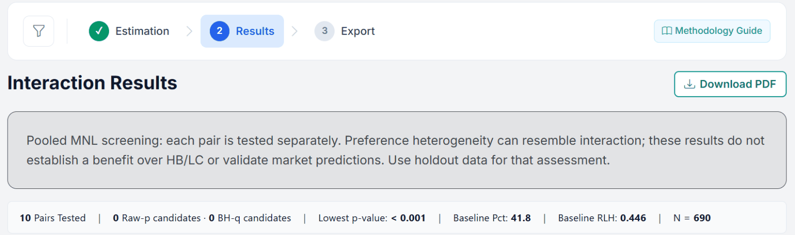
The results view (step 2 Results, headed Interaction Results) opens with a standing note that this is a pooled MNL screening: each pair is tested separately, preference heterogeneity can resemble interaction, and holdout data should decide the final model. Runs created before the current validation checks additionally show a warning asking you to re-estimate them. Below that comes a one-line metrics bar:
Metric
Description
Pairs Tested
Total number of attribute pairs examined
Raw-p candidates · BH-q candidates
Two counts: pairs passing the raw-p decision (p ≤ alpha and Improvement ≥ threshold) and pairs passing the FDR decision (q ≤ alpha and Improvement ≥ threshold)
Lowest p-value
Smallest p-value across all tested pairs (shown as “< 0.001” below that bound)
Baseline Pct
Percent certainty (McFadden ρ²) of the main-effects-only model
Baseline RLH
Root Likelihood (geometric mean predicted probability) of the main-effects model
N
Number of respondents included in the analysis
Figure 3. Top of the results view for the Pizza run IS_CBC_1 (default practical threshold 1.0). No pair is flagged, although the lowest p-value is below 0.001.
In the Pizza run the main-effects model reaches a percent certainty of 41.8 and an RLH of 0.446. Ten pairs were tested; the smallest p-value is below 0.001, yet neither count shows a candidate. The reason is the practical threshold, as section 4.4 explains.
4.2 Level Interaction Explorer
The first card below the metrics bar is the Level Interaction Explorer, subtitled “Inspect pair-level synergies by attribute levels”. Its controls are:
Attribute Pair, a dropdown listing every tested pair. Significant pairs are marked with a “[sig]” suffix and sort to the top; a pair without estimable level effects shows a placeholder note instead of a table.
Top Rows, with Top 8, Top 12 (default) and Top 20. This limit applies to the slope and raw-term tables only; the level-effects table always shows every level pair, and the control is hidden in that case.
Raw-p candidates only (including practical threshold), a switch that restricts the dropdown to pairs flagged by the raw-p decision.
A PNG button in the card header that exports the whole explorer card as an image.
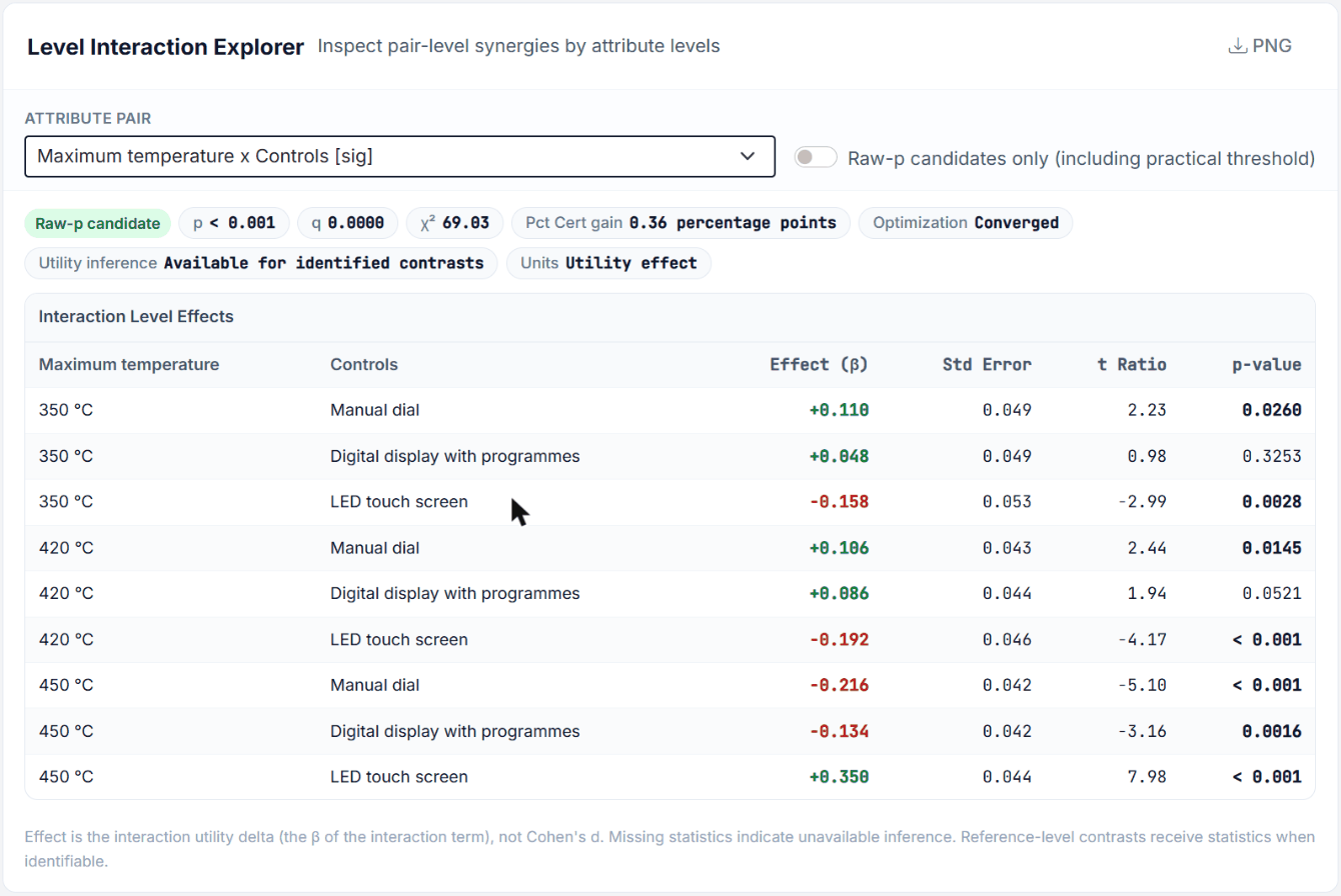
Above the table, a short list shows the result Raw-p candidate, Raw-p criteria not met or Inference unavailable for the selected pair, followed by p, q, χ², the Pct Cert gain in percentage points, the optimization state (Converged or Not converged / not fitted), whether utility inference is available, and the units of the effects shown.
Categorical × Categorical
When both attributes are categorically coded, the explorer shows an Interaction Level Effects table in long format: one row per level combination with the columns attribute A level, attribute B level, Effect (β), Std Error, t Ratio and p-value. Positive effects are shown in green with a plus sign (the combination is valued more than the main effects alone would predict), negative effects in red. The effect is the interaction utility delta, that is the β of the interaction term, not an effect size such as Cohen's d. Reference-level cells implied by effects coding are included and receive standard errors and p-values whenever their contrast is identifiable. A dash marks cells whose inference is unavailable (non-identifiable contrast, or the covariance of the pair model could not be computed); the note below the table explains this.
Categorical × Linear
When one attribute is categorical and the other is linear, the explorer shows a Slope deltas by level table. Each level of the categorical attribute gets its own slope adjustment, showing how the linear effect changes for that level. Rows are sorted by absolute magnitude and limited by the Top Rows setting.
Linear × Linear
When both attributes are linear, the interaction is a single coefficient, the cross-product of the two linear terms, printed as one line.
Figure 4. The Level Interaction Explorer for Maximum temperature x Controls in the Pizza run IS_CBC_2 (practical threshold 0.25).
Pizza example: reading the level effects
The largest effect is 450 °C with LED touch screen: +0.350 (t = 7.98). The hottest oven is worth clearly more when it comes with the touch screen than the two main effects together predict. The other 450 °C combinations are negative (manual dial −0.216, digital display −0.134), and at 350 °C and 420 °C the touch screen loses (−0.158 and −0.192). Read as a pattern: buyers who go for top heat also want the premium control, and the touch screen is not worth extra on a basic oven.
4.3 Interaction Search Summary
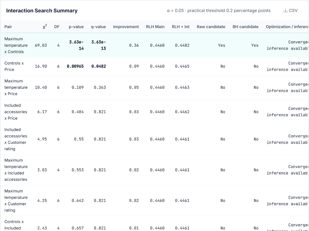
Below the explorer, the Interaction Search Summary card lists every attribute pair. Its header repeats the settings used (“α = 0.05 · practical threshold 0.25 percentage points” in Figure 5) and carries a CSV button that downloads the table as displayed. Pair names are written as “Brand x Price”. The columns are:
Column
Meaning
Pair
The two attributes being tested (e.g., “Brand x Price”)
χ²
Likelihood-ratio test statistic, larger values indicate stronger evidence against the null hypothesis of no interaction
DF
Effective degrees of freedom of the test, the rank gain of the design matrix when the interaction columns are added. With a complete design this equals the product of the coded column counts (see Section 8); with prohibitions or empty cells it can be smaller
p-value
Raw (unadjusted) statistical significance; values below 0.001 are shown as “< 0.001”, the CSV keeps the exact value
q-value
FDR-adjusted p-value using the Benjamini-Hochberg procedure over the tested pairs. A q-value < 0.05 means you can expect at most 5% false discoveries among all pairs declared significant
Improvement
Pct-certainty gain from adding this interaction to the main-effects model (in percentage points)
RLH Main
Root Likelihood of the main-effects-only model
RLH + Int
Root Likelihood after adding this pair’s interaction terms
Raw candidate
Yes if the pair passes the raw-p decision (p ≤ alpha and Improvement ≥ threshold), No otherwise, n/a if inference is unavailable
BH candidate
The same for the FDR decision (q ≤ alpha and Improvement ≥ threshold)
Optimization / inference
Converged when both the baseline and the pair model converged and likelihood-ratio inference is available; Converged; inference unavailable or Not converged / not fitted otherwise
Rows flagged by the raw-p decision get a tinted background, and p- or q-values at or below the configured alpha (0.05 for the default confidence level) are set in bold when inference is available.
Reading the table
Start with the highlighted rows. These are the pairs that passed both hurdles. The table is ordered by p-value; among the highlighted rows, compare the Improvement column to find the pair that contributes the most to model fit (export the CSV if you want to re-sort). Then use the Level Interaction Explorer above to understand the direction of the effect.
Figure 5. The Interaction Search Summary of the Pizza run IS_CBC_2.
With the practical threshold at 0.25, Maximum temperature x Controls is a raw-p and a BH-q candidate. Controls x Price is significant on both p (0.00965) and q (0.0482), but its improvement of 0.09 points stays below the threshold, so it is not flagged. Every other pair has p ≥ 0.109. Section 10 comes back to Controls x Price: it is a typical example of a signal that heterogeneity can produce.
4.4 Significance: Raw p and FDR q
Choicery reports significance two ways, side by side. Both share the same practical-significance requirement, and both additionally require that the baseline model and that pair’s full model converged, that the observed-information matrix of each fit is full rank (no quasi-complete separation), that the interaction model’s log-likelihood is not below the baseline, and that the pair has at least one estimable interaction contrast (effective DF > 0). Pairs failing any of these show “inference unavailable” and n/a instead of a decision:
1
Raw-p decision: p-value ≤ alpha (where alpha = 1 − confidence level). For the default 95% confidence level, alpha = 0.05. This is the flag that drives the row highlight and the Raw-p candidates count in the metrics bar.
2
FDR decision: q-value ≤ alpha, where q comes from the Benjamini-Hochberg correction across all tested pairs. This is the safer guide when many pairs are tested. It is reported in the q-value column and the BH candidate column, drives the BH-q candidates count in the metrics bar, and appears as Significant (FDR q) in the exported workbook.
3
Practical significance (required for both): Improvement ≥ practical threshold. For the default threshold of 1.0%, the interaction must improve pct-certainty by at least 1.0 percentage points.
Requiring a minimum effect size prevents a common trap: with large samples, even trivially small interactions become statistically significant.
Pizza example: the same data, two thresholds
IS_CBC_1 uses the default threshold of 1.0: Maximum temperature x Controls has p < 0.001 but gains only 0.36 points, so the explorer badge reads Raw-p criteria not met and the metrics bar shows 0 candidates (Figure 3). IS_CBC_2 repeats the run with 0.25: the same pair becomes a raw-p and BH-q candidate, everything else is identical. The threshold does not change the test, only which pairs are flagged. Choose it before you look at the results, and report it.
Why the effect-size hurdle matters
In a study with 1,000 respondents, you might find that Brand x Color has p < 0.01 but an improvement of only 0.08 percentage points. This interaction is statistically “real” but practically irrelevant, it explains almost no additional variation. Requiring the practical threshold correctly excludes it.
4.5 Inestimable Pairs
Prohibited level combinations can leave some interaction cells empty. Their columns are then collinear with the main effects and carry no information. Choicery detects this from the rank of the design matrix:
If all interaction columns of a pair are collinear, the pair is inestimable. It is reported with DF 0 and no test statistics (χ², p-value and q-value show n/a, and so do the Raw candidate and BH candidate columns), is never flagged significant, and is excluded from the Benjamini-Hochberg family so it cannot dilute the correction.
If only some columns are collinear, the pair is partially estimable and the chi-square test uses the reduced effective degrees of freedom.
Both cases are visible in the DF column and the Optimization / inference column of the summary table, in the Managerial Summary sheet and the per-pair sheets of the Excel workbook (nominal versus effective degrees of freedom), and as inestimable_count and partially_estimable_count in the results JSON.
5. Exporting Results
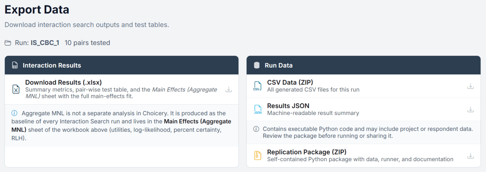
Step 3 Export is headed Export Data and groups the downloads into two cards, Interaction Results and Run Data:
Export
File
Contents
Download Results (.xlsx)
Interaction_Search_<run name>.xlsx
Sheets: Summary (one row per model: Main Effects and each “+ pair”, with parameters, log-likelihood, chi-square, p-value, gain in pct certainty, FDR q-value, Significant (raw p), Significant (FDR q)), Settings Summary, Managerial Summary (plain-language interpretation and caveats), Charts (a ranked table of the significant pairs with p, q, gain and χ²; empty when no pair is significant), Main Effects (Aggregate MNL) with the full baseline fit, and one sheet per attribute pair
CSV Data (ZIP)
Interaction_Search_Data_<run name>.zip
All generated CSV files for the run, including Interaction_Search_Summary.csv, Interaction_Coefficients.csv, Interaction_Main_Effects.csv and the converted choice data
Results JSON
interaction_results_<run id>.json
Machine-readable result summary for programmatic access
Replication Package (ZIP)
Interaction_Replication_<run name>.zip
Self-contained Python package with data, runner and documentation for offline validation
The Aggregate MNL model is not a separate analysis in Choicery. It is produced as the baseline of every Interaction Search run and lives in the Main Effects (Aggregate MNL) sheet of the workbook (utilities, log-likelihood, percent certainty, RLH). The downloads page states this explicitly.
Replication package
The replication package is useful for peer review, auditing, or sharing results with collaborators who do not have access to your Choicery project. It contains executable Python code and may include project or respondent data, so review it before running or sharing it. Only the confidence level, practical threshold, max iterations and convergence tolerance can be changed in the packaged runner; coding and None handling are frozen with the source run, and package results cannot be imported back into Choicery. If the run has no complete, verified estimator snapshot (for example a run created before snapshots were introduced) or the snapshot exceeds 100 MB, the entry is shown locked with the reason; re-run the analysis to create a package. Downloading the package also requires the analysis-package feature of your plan.
Two more exports sit outside the Export step:
Download PDF in the header of the Results step, which renders the interaction results as a PDF report.
The CSV and PNG buttons inside the results cards, which export the summary table and the explorer card as displayed.
Figure 6. The Export step of the Pizza run IS_CBC_1.
6. Best Practices & Common Pitfalls
Do:
Treat Interaction Search as the screening step it is. It tells you which pairs would be worth modeling explicitly, rather than guessing. Note that Choicery’s in-app Preference Analysis (HB) estimates main effects only; there is no checkbox for adding attribute interaction terms. Acting on a finding therefore means changing the study design (for example moving to conditional pricing) or re-specifying the model outside Choicery.
Use the default practical threshold (1.0%) to filter out trivially small effects. Adjust only if you have a specific reason.
Check if “significant” interactions disappear when using HB with heterogeneity. Many aggregate interactions are actually heterogeneity artifacts (Orme & Williams, 2016: only 4 of 22 commercial datasets benefited from explicit interaction terms).
Focus on substantively interpretable interactions. Brand × Price is common and meaningful. Color × Warranty might be statistically significant but hard to explain, be skeptical of such pairs.
Use the Level Interaction Explorer to understand the direction of the effect, not just its existence.
Don’t:
Don’t add ALL significant interactions to your model. Start with the strongest 1 or 2 and evaluate model improvement. Adding too many interaction terms increases model complexity and can lead to overfitting.
Don’t panic if you find many significant interactions. With large samples, even trivial effects become “significant.” Always check the Improvement column.
Don’t use Interaction Search with very small samples (<50 respondents). The aggregate MNL may not converge reliably, and low statistical power means you will miss genuine interactions.
Don’t confuse statistical significance with practical importance. Always check the Improvement column alongside the p-value.
Don’t forget: this test uses an aggregate MNL, not HB. Results show population-average interactions. Some of what appears as an interaction may be a heterogeneity artifact, a pattern that arises because different segments have different main effects, not because of a true within-person interaction.
The heterogeneity trap
If half your respondents love Brand A and hate Brand B, while the other half feels the opposite, an aggregate model will show no brand effect. But if these groups also differ in price sensitivity, the aggregate model may compensate by finding a Brand × Price interaction that does not exist at the individual level. Always cross-check aggregate interaction results against HB individual-level outputs.
Part II
Theoretical Background
Statistical foundations, model structure, and the methodological considerations behind Interaction Search.
7. Key Definitions
Glossary
Interaction Effect
A situation where the preference for a level of attribute A depends on which level of attribute B is present. Formally, the joint utility of levels a and b differs from the sum of their individual (main-effect) utilities.
Additive Main-Effects Model
A model in which the total utility of a product profile is the sum of the individual attribute-level utilities: U(profile) = ∑ U(levelk). This is the standard assumption in most conjoint analyses.
Likelihood-Ratio Test (2ΔLL)
A chi-square test that compares two nested models by examining the difference in their log-likelihoods. If the fuller model (with interaction terms) fits significantly better than the restricted model (main effects only), the interaction is deemed statistically significant.
Benjamini-Hochberg FDR
A multiple-comparison correction that controls the false discovery rate, the expected proportion of false positives among all rejected null hypotheses. Less conservative than Bonferroni, it provides greater statistical power while still controlling the overall error rate.
Pct Certainty (McFadden ρ²)
A goodness-of-fit measure for discrete choice models, defined as (1 − LLmodel / LLnull) × 100. Values range from 0 (model no better than chance) to 100 (perfect prediction). Even small values (5 to 15%) indicate meaningful model fit in conjoint contexts.
Root Likelihood (RLH)
The geometric mean of the predicted probabilities for the chosen alternatives across all choice tasks. An RLH of 0.50 for a 4-alternative design means the model predicts twice as well as random chance (which would yield 0.25).
Effects Coding
A design-matrix coding scheme in which the reference level is set to the negative sum of all other levels, rather than zero (as in dummy coding). This ensures that main effects are interpretable as deviations from the grand mean, and in balanced designs it keeps interaction columns separate from the main-effect columns. Choicery checks estimability by the rank of the design rather than assuming orthogonality.
Cross-Product Terms
Interaction columns in the design matrix created by multiplying the main-effect columns of two attributes element-wise. For effects-coded attributes A (with columns a1, …, ap) and B (with columns b1, …, bq), the cross-product terms are ai × bj for all i, j combinations.
8. The Statistical Test
8.1 Aggregate MNL Baseline Model
Choicery first estimates a main-effects-only multinomial logit (MNL) model on the pooled (aggregate) choice data. This model assumes that all respondents share the same preference weights and that attribute effects are additive:
P(i | Ct) = exp(Vi) / ∑j ∈ Ct exp(Vj)
MNL choice probability: alternative i from choice set Ct
Vi = ∑k βk · xik
Systematic utility: sum of main effects only
The model is estimated by maximizing the log-likelihood over all observed choices. This gives the baseline log-likelihood LLmain.
8.2 Full Model with Interaction Terms
For each attribute pair (A, B), Choicery estimates a second model that includes all main effects plus the cross-product terms for that specific pair:
Vi = ∑k βk · xik + ∑p, q γpq · (xiAp · xiBq)
Utility with main effects + interaction terms for pair (A, B)
This gives LLfull for each pair. Since the interaction model nests the main-effects model (setting all γpq = 0 recovers the baseline), the likelihood-ratio test applies.
8.3 Likelihood-Ratio Test
χ² = 2 × (LLfull − LLmain) ~ χ²(df)
Likelihood-ratio test statistic, asymptotically chi-square distributed
Under the null hypothesis (no interaction), this statistic follows a chi-square distribution with df degrees of freedom, where df equals the number of additional parameters in the interaction model.
8.4 Degrees of Freedom by Coding Type
The number of additional parameters (and hence the degrees of freedom for the chi-square test) depends on how each attribute is coded:
Under effects coding, an attribute with L levels is represented by L − 1 columns (the last level is the negative sum of the others). This means the number of interaction parameters equals the product of the coded column counts, not the product of the level counts. This keeps the interaction model parsimonious.
Nominal versus effective degrees of freedom
The table above gives the nominal df. Choicery tests against the effective df instead, computed as the rank gain of the design matrix when the interaction columns are added. With a complete design the two are identical. When prohibitions or empty level combinations make some interaction columns collinear with the main effects, the effective df is smaller, and using the nominal df would bias the p-value conservatively. The DF column in the results table shows the effective value.
9. Multiple Comparison Correction
9.1 The Problem
When testing multiple attribute pairs simultaneously, the probability of at least one false positive increases rapidly. With k attributes, you test k(k − 1) / 2 pairs. At α = 0.05, the expected number of false positives is 5% × number of tests.
Example: False positive inflation
With 8 attributes, you test 28 pairs. Even if no true interactions exist, you expect 28 × 0.05 = 1.4 false positives on average. This means there is a high probability that at least one pair will appear “significant” by chance alone.
9.2 Bonferroni Correction
The simplest approach: divide the alpha threshold by the number of tests. For 28 tests at α = 0.05, the Bonferroni-adjusted threshold becomes 0.05 / 28 = 0.00179. This controls the family-wise error rate (the probability of any false positive), but is very conservative, it substantially reduces power to detect true interactions.
9.3 Benjamini-Hochberg (Used by Choicery)
Choicery uses the Benjamini-Hochberg (BH) procedure (Benjamini & Hochberg, 1995), which controls the false discovery rate (FDR) rather than the family-wise error rate. The FDR is the expected proportion of false positives among all discoveries (rejected nulls).
The procedure works as follows:
1
Rank all m p-values from smallest to largest: p(1) ≤ p(2) ≤ … ≤ p(m).
2
For each rank i, compute the BH critical value: (i / m) × α.
3
Find the largest rank i for which p(i) ≤ (i / m) × α. Reject all null hypotheses with rank ≤ i.
The resulting q-values (adjusted p-values) represent the minimum FDR at which each pair would be declared significant. A q-value < 0.05 means: if you call this pair significant, you can expect that at most 5% of all your “significant” calls are false discoveries.
In Choicery, m is the number of design-testable pairs (effective DF > 0). Inestimable pairs (see Section 4.5) are left out of the family, so they cannot inflate m and weaken the correction for the pairs that were tested. Pairs that are design-testable but whose fit failed (no likelihood-ratio inference) stay in the family and enter the correction with an internal p-value of 1, which is conservative for the other pairs; their own q-value is shown as n/a.
9.4 Worked Example
Pizza example: 5 attributes, 10 pairs, α = 0.05
The three smallest p-values of the Pizza run are:
Rank Pair p-value BH threshold (i/10 × 0.05)
1 Maximum temperature × Controls 3.6e-14 0.005 ← passes ✓
2 Controls × Price 0.00965 0.010 ← passes ✓
3 Maximum temperature × Price 0.109 0.015 ← fails ✗
The first two pairs survive the correction; their q-values are 3.6e-13 and 0.0482 (q(i) = p(i) × m / i, made monotone from the largest rank down). Controls × Price passes with little room to spare: with 20 pairs instead of 10 its q-value would double to about 0.097 and it would fail.
Choicery then applies the practical threshold. At 1.0 neither pair is flagged; at 0.25 only Maximum temperature × Controls (0.36 points) is, while Controls × Price (0.09 points) stays below it (section 4.4).
10. The Heterogeneity Caveat
This is perhaps the most important methodological consideration for Interaction Search, and one that is frequently overlooked.
Critical insight from Orme & Williams (2016)
Many apparent interactions found in aggregate (pooled) models are not true within-person interaction effects. They are heterogeneity artifacts, statistical shadows cast by unrecognized preference segments that differ in their main effects.
Consider the following scenario:
Example: Heterogeneity masquerading as interaction
A study has Brand (A, B) and Price ($10, $20, $30). The sample contains two latent segments:
Segment 1 (50%): Loves Brand A, very price-sensitive
U(A) = +2.0, U(B) = -2.0, Price slope = -0.15 per $
Segment 2 (50%): Loves Brand B, price-insensitive
U(A) = -1.5, U(B) = +1.5, Price slope = -0.02 per $
When you pool these two segments and estimate an aggregate MNL, the average brand effects nearly cancel out and the average price slope is moderate. But the aggregate model “discovers” a Brand × Price interaction: Brand A appears more price-sensitive than Brand B. This is not a true interaction, it is a correlation between brand preference and price sensitivity across segments.
Pizza example: Controls × Price
In the Pizza run Controls × Price passes the FDR correction (q = 0.048) with a tiny improvement of 0.09 points. The Latent Class guide finds a matching segment structure in the same task: the only segment that cares about the controls is on average 70 years old and also the one with the highest lay rationalism, the trait that makes people weigh price more. When the people who care about the controls also differ in price sensitivity, the pooled model can show a Controls × Price signal without any respondent valuing the price differently depending on the controls. The level pattern of Maximum temperature × Controls (Figure 4) is a more convincing candidate: it is large, specific and makes sense product-wise.
The key finding from Orme and Williams (2016) is striking: in an analysis of 22 commercial conjoint datasets, only 4 datasets showed genuine interactions that improved HB model fit when explicit interaction terms were added. The remaining apparent interactions in aggregate models were adequately captured by HB’s individual-level heterogeneity.
Practical implications
Use Interaction Search as a screening tool, not as definitive proof. If a pair is significant in the aggregate test, verify by examining HB individual-level utilities.
If the interaction disappears when you look at HB utilities across segments (e.g., via Latent Class), it was likely a heterogeneity artifact.
True interactions persist at the individual level. For example, in conditional pricing designs (where each brand has its own price range), a Brand × Price interaction is real because the price meaning genuinely differs by brand.
Rule of thumb
If an interaction is significant in the aggregate Interaction Search but disappears when you look at HB utilities across Latent Class segments, it is almost certainly a heterogeneity artifact. True interactions show up consistently at the individual level.
11. When to Add Interactions to Your Model
Given the heterogeneity caveat, when should you actually add interaction terms to your conjoint model? Here are practical guidelines:
Scope note
This section is methodological guidance. Choicery’s in-app Preference Analysis (HB) estimates main effects only, so the estimation steps below refer to a model you specify yourself in your own estimation code (the replication package ships the run data and a Python runner as a starting point). What you can act on inside Choicery is the study design (conditional pricing, prohibitions) and the decision whether to interpret and simulate on main effects alone.
Scenario
Recommendation
Rationale
Conditional pricing (brand-specific price ranges)
Almost always add
Price meaning genuinely differs by brand, creates real within-person interactions
Brand × Price (common price levels)
Investigate carefully
Common and often genuine, but can also be a heterogeneity artifact
Improvement > 2% pct-certainty
Worth investigating
Large effects are more likely to reflect genuine interactions
Improvement 0.5% to 2%
Proceed with caution
Check HB holdout prediction, does the interaction model predict better?
Improvement < 0.5%
Usually ignorable for overall fit
Too small to change the model as a whole. Still look at the level effects: a strong, specific pattern (the Pizza pair gains 0.36 points with t = 7.98 for one combination) can matter for one product
Validation approach
If you decide to add interaction terms to your HB model, validate the decision with holdout tasks:
Estimate HB with main effects only. Record holdout hit rate.
Estimate HB with main effects + the interaction. Record holdout hit rate.
If the interaction model improves holdout prediction, the interaction is likely genuine and worth keeping.
If holdout prediction stays the same (or decreases), the interaction is likely a heterogeneity artifact that HB already handles through individual-level estimation.
Start small
If multiple pairs are significant, add them one at a time, starting with the strongest. Adding too many interactions at once increases model complexity, can cause estimation instability, and makes interpretation difficult.
12. References
Benjamini, Y., & Hochberg, Y. (1995). Controlling the false discovery rate: A practical and powerful approach to multiple testing. Journal of the Royal Statistical Society: Series B, 57(1), 289-300.
Louviere, J. J., & Woodworth, G. (1983). Design and analysis of simulated consumer choice or allocation experiments. Journal of Marketing Research, 20(4), 350-367.
Orme, B. K. (2020). Getting started with conjoint analysis (4th ed.). Manhattan Beach, CA: Research Publishers LLC.
Orme, B. K., & Chrzan, K. (2017). Becoming an expert in conjoint analysis. Orem, UT: external conjoint software.
Orme, B. K., & Williams, J. (2016). Interaction effects in conjoint analysis: A cautionary note [Research paper]. Orem, UT: external conjoint software.
Rao, V. R. (2014). Applied conjoint analysis. Berlin: Springer.