How to discover profile-driven preference heterogeneity using neural-embedded discrete choice models, Hybrid TasteNet, and Neural-HB MAP. Every setting of the form, how to read the results, and the method behind it, with the pizza oven CBC of the Pizza (Example) study as worked example. Based on the TasteNet-MNL model (Han et al., 2022).
Everything you need to run, interpret, and export the AI-Driven Profile Analysis in Choicery.
1. What Is the AI-Driven Profile Analysis?
TasteNet discovers how and why respondents differ in their preferences. Unlike HB estimation, which tells you what each person’s preferences are but not why they differ, TasteNet uses a neural network to learn the relationship between respondent characteristics (age, income, attitudes) and their conjoint preferences.
The core idea is deceptively simple: instead of estimating preference weights independently for each respondent (as HB does), TasteNet learns a function that maps respondent covariates to preference weights:
βi = NeuralNetwork(covariatesi)
The neural network takes a respondent’s survey answers as input and outputs their individual preference weights.
TasteNet is based on the neural-embedded discrete choice model proposed by Han, Pereira, Ben-Akiva, and Zegras (2022) at MIT and DTU. It retains the economic interpretability of the multinomial logit model while allowing the taste parameters to be learned as nonlinear functions of respondent characteristics.
The core idea
HB tells you that Person A strongly prefers Brand X while Person B cares mostly about price. TasteNet goes further: it tells you that younger, urban respondents with high tech-affinity scores tend to prefer Brand X, while older, price-conscious respondents prioritize cost. TasteNet connects the what to the why.
Key Output
Individual-level utilities, like HB, every respondent gets their own preference weights.
Covariate importance rankings (SHAP), which respondent characteristics most influence preferences, and in what direction.
Group comparison charts, visual breakdowns showing how preferences differ across demographic or attitudinal groups (e.g., “Age 18-29 vs. 50+”).
Persona Simulation, TasteNet enables the Persona tab in the Market Simulator, which lets you create hypothetical consumer profiles from covariate values and instantly see their predicted preferences and choice probabilities, without these personas ever having taken the survey.
The Unique Advantage: Predicting Preferences for New People
Because TasteNet’s utilities are a deterministic function of covariates (βi = NN(zi)), you can predict the preferences of anyone whose covariate profile you know, even if they never participated in the conjoint study. Define a “persona” (e.g., female, age 35, high income, strong sustainability attitude) and TasteNet instantly produces her predicted utility profile.
This is NOT possible with HB
HB estimates individual utilities using both covariates AND a respondent-specific random effect (βi = XiΓ + ui). The random effect ui is estimated from each person’s actual choice data via MCMC. For someone who never took the survey, there is no choice data to compute ui, you would only get the covariate-adjusted population mean, not a true individual prediction. TasteNet has no random effect: all individual variation is explained by covariates, making out-of-sample prediction possible.
Persona Simulation in Choicery
The Persona tab in the Market Simulator (only available after a TasteNet run) lets you define hypothetical consumer profiles, predict their preferences, and simulate their market choices. This is especially valuable for targeting: “What would a 25-year-old male tech enthusiast choose?”, answered without that person ever being in your sample.
Why TasteNet Instead of Just HB?
HB can also include covariates, Choicery supports upper-level covariate effects in HB estimation (via the Create Package option). However, HB’s covariate model is linear: it assumes each covariate shifts the population mean by a fixed amount. TasteNet’s neural network learns nonlinear, interaction-rich covariate-preference mappings automatically, for example, that age affects price sensitivity differently for high-income vs. low-income respondents, without the analyst specifying this interaction. Additionally, SHAP provides a principled decomposition of covariate importance that goes beyond linear coefficient tables.
TasteNet vs. HB with covariates
Both HB and TasteNet can use respondent covariates. The difference: HB’s upper-level covariate model is a linear regression on the population mean (each covariate shifts μ by a constant), plus an individual random effect estimated from choice data. TasteNet uses a neural network that can discover nonlinear effects and covariate interactions automatically, with no random effect, all heterogeneity is explained by covariates. For simple covariate relationships, HB covariates are sufficient. For complex relationships, out-of-sample prediction, or Persona simulation, TasteNet is the right choice.
What Is Neural-HB? (Start Here if You Know HB)
Neural-HB is a Choicery-specific estimator. You will not find the name in textbooks or other conjoint tools: it was developed for Choicery to combine the two ideas above. Conceptually it is a hierarchical model whose upper level is a neural network; in the literature it corresponds to a mixed logit with a nonlinear concomitant-variable prior mean, estimated as a Laplace-initialized variational posterior (a MAP fit with a learned local Gaussian around it, not MCMC; “Neural-HB MAP” in older material and the internal setting name refer to the same estimator) (Section 12.13 gives the formal treatment).
The easiest way to understand it is as a three-step ladder:
Model
The anchor an individual’s utilities are pulled toward
Individual deviations from that anchor?
Classic HB
One shared population mean
Yes, estimated from each respondent’s own choices
TasteNet
A personal covariate prediction NN(zi)
No, covariates explain everything
Neural-HB
A personal covariate prediction NN(zi)
Yes, HB-style shrunken deltas δi from each respondent’s own choices
In words: Neural-HB keeps TasteNet’s neural network as a personalized population mean and then, exactly like HB, lets every respondent deviate from that mean where their own choices demand it. The deviations are shrunken toward zero (the delta L2 per task setting in 3.6 controls how strongly), so respondents with little or noisy data stay close to what their profile predicts, while consistent individual choice patterns pull them away from it.
What a Neural-HB run gives you:
Full individual utilities, like HB. Each respondent’s exported utility is the neural prediction plus their individual delta. The Results export mirrors the familiar HB report (Summary, Settings & Diagnostics, Individual Utilities ZC, ...), and observed respondents can be simulated with their full utilities.
The TasteNet explanation layer on top. SHAP and the covariate views explain the neural component: which profile variables shape preferences, and how.
A heterogeneity decomposition (on the Results page and in the Technical Diagnostics workbook) showing, per utility, how much of the preference variation the profile explains and how much is individual residual taste.
Rule of thumb
Care mainly about individual utilities and simulation accuracy for your sample? Classic HB remains the default. Care mainly about why preferences differ and about scoring new profiles? TasteNet. Want both at once, individual utilities and a nonlinear covariate story? That is Neural-HB.
2. Prerequisites
Before running TasteNet in Choicery, make sure you have the following:
1
A conjoint task with collected responses. TasteNet supports all conjoint types available in Choicery: CBC, CBC Shop, DR-CBC, BW-CBC, MaxDiff, and Anchored MaxDiff. The conjoint task and its experimental design must already exist in your project.
2
At least ~200 respondents (recommended). Neural networks require more data than Bayesian methods. While TasteNet can technically run with fewer respondents, results become unreliable below ~150. For stable SHAP importance rankings, 300+ respondents are ideal.
3
Survey variables collected as covariates. Standard TasteNet requires covariates: the Covariates panel carries a Required badge and the run will not start without at least one selected variable. You need at least 3-5 variables measuring demographics, attitudes, or behaviors. These are the respondent characteristics that TasteNet will use to predict preference heterogeneity.
4
Open the tab. Header menu Analysis → Conjoint Analysis, pick the task in the sidebar under Analysis Tasks, then the second tab AI-Driven Profile Analysis (on narrow screens "AI-Profile"; greyed out with "Task specific" where a task type is not supported). Below the tabs sits the strip Estimation → Results → Export.
Covariates are mandatory for standard TasteNet
Unlike HB or LC, standard TasteNet cannot run without covariates. Without respondent-level characteristics as input, the neural network has nothing to learn from, and TasteNet collapses to an aggregate MNL model. Always include meaningful covariates.
The one exception is the Neural-HB switch. When it is on, the badge next to the Covariates label changes from Required to Optional and the panel reads “Optional: Neural-HB will use an intercept-only mean and respondent-level residuals.” That configuration gives up the covariate explanation layer entirely, so it is only sensible when you want the individual-level utilities and nothing else.
3. Running TasteNet in Choicery
3.1 Creating a Run
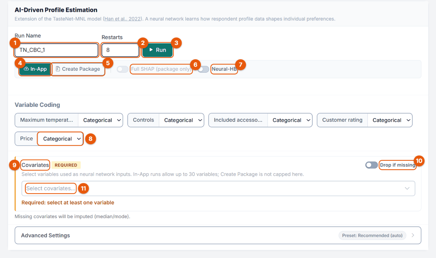
Each estimation is saved as a named run, so you can compare configurations and results. Figure 1 shows the form of the Pizza oven CBC (cbc_pizza_oven, 690 respondents).
Figure 1. The AI-Driven Profile Estimation form (Pizza task cbc_pizza_oven).
No.
Control
What it does
1
Run Name
Label of the run, suggested as TN_CBC_1, TN_CBC_2 ... Rename it to something meaningful, e.g. TN_4cov.
2
Restarts
How many times the network is trained from new random starting weights; the restart with the best internal validation loss is kept. The preset suggests a value for your sample size (8 for the 690 Pizza respondents). In-App up to 20 (40 with Neural-HB), Create Package up to 100.
3
Run
Starts the estimation (section 3.7).
4
In-App
Trains on the Choicery server; results appear in Results by themselves.
5
Create Package
Builds a Python package for your own computer (section 3.5). Then a Samples field for bootstrap confidence intervals appears.
6
Full SHAP (package only)
Expanded SHAP with larger samples. Only usable with Create Package; greyed out In-App, where the fast SHAP variant runs.
7
Neural-HB
Switches to the Neural-HB estimator (section 1 and 3.5): the network becomes a personal prior mean and every respondent gets an own deviation. Adds two fields (delta L2 per task, Final refit epochs) and makes covariates optional.
8
Variable Coding
Categorical or Linear per attribute, as in HB (section 3.4).
9
Covariates (Required)
The respondent characteristics the network learns from (section 3.2).
10
Drop if missing
Off: missing covariate values are imputed (median for numbers, most frequent category otherwise). On: respondents with a missing value are left out.
11
Select covariates...
Opens the variable picker with search and type tags.
Why multiple restarts matter more for TasteNet than for HB
HB is a Bayesian MCMC sampler, given enough draws, chains converge to the same posterior regardless of starting values. TasteNet minimizes a non-convex loss with gradient descent, so local minima are real. Pachali, Kurz & Otter (2020) also caution that neural choice models estimated with few restarts can produce unstable individual-level estimates. Run at least 5 restarts in-app, or 20-50 in the offline package, and compare validation RLH across restarts to judge stability.
Run Name: up to 50 characters and unique per task ("Run name '...' is already in use.").
Samples (Create Package only): bootstrap refits for confidence intervals, default 100, up to 5,000. 0 (no bootstrap) is allowed for Neural-HB packages only; standard TasteNet packages need at least 1.
Run bar: above the card, the Run: dropdown lists saved runs (with a trash icon each), shows "Current data N = ..." or the N of the selected run, and offers New Run on finished runs, whose form is then locked. At most 10 runs per task ("Maximum of 10 TasteNet runs per task reached. Delete a run before starting a new one."). Failed and cancelled runs say so ("Run failed.", "This run was cancelled.").
3.2 Selecting Covariates (Required)
The Covariates panel is the defining feature of TasteNet: these are the respondent variables the neural network will learn to map into utilities. You must select at least one covariate; 5-15 is the recommended range.
Figure 2. Four covariates selected for the Pizza run: two z-standardized attitude scales, age and gender.
For the Pizza study, sensible covariates are the respondent characteristics that plausibly shape what someone wants from a pizza oven: food_involvement_z (how much someone cares about food), lay_rationalism_z (how strongly someone decides by "hard" facts such as price), age and gender. Single items of a grid or open answers are usually poor inputs; use scale scores where you have them.
Both numeric variables (age, income, Likert scores, usage frequency) and categorical variables (gender, region, education, occupation) are supported. The picker tags each variable as Metric, Ordinal or Nominal (from the variable configuration; Likert items count as metric). By default each metric covariate enters the network as one standardized (z-scored) column; nominal and ordinal covariates are dummy coded: one 0/1 column per category except a reference category, which is recorded in the run metadata. Text answers, conjoint items, constant columns and system or timing columns are not offered; columns added in the Data Editor are. The raw column names, dtypes, and preprocessing metadata are preserved so that later profile-based prediction (Section 14) works for any new respondent vector on the same scale.
The optional Smooth numeric covariate effects setting changes only that first step. Instead of one column, each metric covariate enters as a small quadratic B-spline basis with four knots placed on training-sample quantiles, continued linearly outside the observed training range. The network can then express a curved effect such as “steep up to 35, flatter afterwards” directly at the input layer rather than having to build the curvature out of hidden units, which the regularization otherwise penalizes. Knots and scaling are learned from training respondents only, so a respondent holdout stays untouched by the encoding. Categorical covariates and the product attributes are unaffected. A variable with too few distinct training values falls back to the standard single column on its own; the run records both the requested and the applied encoding. The setting applies to plain TasteNet, Neural-HB and the generated replication packages alike.
The Drop if missing toggle governs missing-value policy. When off, median (numeric) or modal (categorical) imputation is applied before training; when on, respondents with any missing covariate are removed from the estimation sample. Imputation keeps sample size but can attenuate effects for sparsely observed variables; dropping is cleaner but costs statistical power.
Covariate selection tips
Include 5-15 covariates for best results. Too few (<3) and TasteNet cannot differentiate respondents, it collapses toward an aggregate model. Too many (>20) with small samples risk overfitting. Attitudinal items (e.g., “How important is sustainability to you?”) often predict preferences better than demographics alone.
3.3 Covariate Groups
There is no group-definition panel in the estimation form. Respondent groups for the group comparison views are derived automatically from the covariate metadata after the run:
Nominal and ordinal covariates: one group per observed level.
Metric covariates: three respondent groups split at z = ±0.5 standard deviations. The labels lead with the back-translated raw value and put the SD boundary in parentheses, for example “< 36.9 (< -0.5 SD)”, “36.9 to 51.2 (-0.5 to +0.5 SD)”, “> 51.2 (> +0.5 SD)”.
Display only: the groups exist for reporting. The neural network always trains on the original continuous values.
Minimum size: groups with fewer than 10 respondents are omitted from the comparison views; the run records how many groups and respondents were skipped.
3.4 Variable Coding
Variable coding determines how conjoint attribute levels are parameterized. This works the same as in HB estimation:
Categorical (default): Each attribute level gets its own part-worth utility. Use this for nominal attributes (e.g., Brand, Color).
Linear: A single slope parameter for ordered/numeric attributes (e.g., Price). Use this when you expect a monotonic relationship.
As soon as at least one attribute is set to Linear, a Sign Constraints block appears underneath with one dropdown per linear attribute:
No sign constraint: the coefficient can be positive or negative.
Positive (>= 0): forces a non-negative coefficient (for example, more features raises utility).
Negative (<= 0): forces a non-positive coefficient (for example, higher price lowers utility).
The form order is Variable Coding, Estimate Display Position Effects (CBC Shop), Include None Option, Sign Constraints, Covariates; MaxDiff and Anchored MaxDiff have no Variable Coding. Include None Option (on by default; DR-CBC, and BW-CBC designs with a none option) adds the follow-up no-choice signal to the model; switch it off to estimate from the product-choice stage only. Estimate Display Position Effects (CBC Shop only) adds technical control terms for the rendered product order. In-App runs accept at most 30 covariate variables; Create Package has no cap. Each task keeps at most 10 saved runs.
3.5 In-App vs Create Package
Choicery offers two execution modes, selected via the pill toggle at the top of the form. Both modes share the same TasteNet-MNL architecture and produce identical result files for the core statistics, the difference lies in where the training runs, which capabilities are unlocked, and how results are brought back into the platform.
At a glance
Aspect
In-App
Create Package
Where it runs
Choicery server (shared resources)
Your own machine (local Python 3.11 or newer)
Results destination
Auto-populated into the Results tab when training finishes
Produces a ..._IMPORT_INTO_CHOICERY.zip which you re-upload into the same run
Restarts
Up to 20 (standard) / 40 (Neural-HB)
Up to 100; no server timeout
SHAP
Fast (sampled, subsampled background set)
Expanded Gradient SHAP / expected gradients with larger evaluation and background samples
Neural-HB
Available (Fast SHAP; up to 40 restarts, 10,000 epochs)
Launchers: install the pinned dependencies and start training (GPU is used automatically with a CUDA-enabled PyTorch)
README.md, MANIFEST.json
Package overview and file manifest
Running it locally
Unzip the package anywhere on your machine.
Install Python 3.11 or newer and, optionally, a CUDA-enabled PyTorch build for GPU acceleration.
Run the launcher: double-click run.bat (Windows) or ./run.sh (macOS/Linux). In a Neural-HB package the launcher starts the Neural-HB trainer; run_baseline.bat / run_baseline.sh start the plain TasteNet comparison instead. On Windows the window stays open at the end and shows whether the run finished. The launcher installs the pinned dependencies into your active Python environment and starts training with the same hyperparameters you configured in-app. If you prefer an isolated environment, run _docs/setup_venv.bat / setup_venv.sh first. The trainer uses the GPU automatically when a CUDA-enabled PyTorch build is installed. On Windows the Neural-HB trainer can ask whether to use multiple CPU cores; accepting uses a conservative core count so the laptop remains responsive.
When training finishes, the script writes its full output into results/ and packs the importable subset into a flat ZIP named after the package folder plus the suffix _IMPORT_INTO_CHOICERY.zip, placed in the package root. This includes: individual utilities, SHAP values, loss history, holdout prediction files, training diagnostics, and if enabled, hybrid residual factors, Neural-HB MAP components, and bootstrap CI tables.
Re-importing results into Choicery
Import workflow
Go back to the AI-Driven Profile Analysis tab for the same task, the run you created carries an External Package badge next to an Import Estimated Data button.
Click Import Estimated Data and pick the ..._IMPORT_INTO_CHOICERY.zip. After a first import the same button reads Re-Import Estimated Data.
Choicery validates the bundle: only files on a fixed allowlist of result basenames are accepted, and tn_results.json plus Individual_Utilities_Raw.csv must be present. Everything else (SHAP tables, holdout predictions, loss history, hybrid and Neural-HB files) is optional and skipped with a warning when missing. The utilities are then merged into the same run.
All downstream TasteNet views unlock: Covariate Importances, Preference Curves by Covariate, Individual Covariate Contributions, Covariate Effect Overview, Group Comparison, Holdout Validation, and, if Hybrid or Neural-HB is enabled, diagnostics separating the covariate-driven neural component from respondent-specific refinement.
Because the utilities are merged into the same run, the Market Simulator and WTP views that use TasteNet utilities work unchanged.
Keep the pair together
The ZIP you re-upload must come from the package Choicery generated, the import validator checks that attribute names, level counts, covariate column names, and respondent IDs match the stored configuration. Editing run_tastenet_bootstrap.py to change architecture, add a custom regularizer, or extend SHAP settings is fine (that is the point of the offline mode), but don’t alter the data files or the run metadata.
Hybrid Random Effects (legacy, superseded by Neural-HB MAP)
An earlier package option, Hybrid Random Effects, added a structured respondent residual on top of the covariate mapping (βn = fθ(zn) + B·hn). It has been hidden from the UI and superseded by Neural-HB MAP below. The backend code is retained so that older runs still load. Section 12 documents the theory for completeness. Hybrid Random Effects is a legacy package-only option; Neural-HB MAP is the current actively supported equivalent in-app and in packages.
Neural-HB MAP
Neural-HB MAP, labelled simply Neural-HB on the switch in the options bar, is the more HB-like estimator. It keeps the neural network as the population-level prior mean, but adds a respondent-specific deviation that is learned from that respondent's own choice history:
βn = fθ(zn) + δn, δn ∼ Normal(0, Σ)
Neural prior mean + respondent-specific MAP deviation. The exported utilities use the full sum; SHAP explains only fθ(z).
The practical motivation is simple: standard TasteNet is excellent for explaining observed covariate structure, but its fit can be weak when the selected covariates do not explain much. Full HB recovers individual utilities from choice histories, but its covariate layer is usually linear. Neural-HB MAP combines the two ideas: a nonlinear neural prior mean for covariate effects, plus HB-style individual shrinkage toward that mean.
This makes Neural-HB useful when the goal is higher observed-respondent utility recovery while still retaining a neural covariate explanation. It should not be confused with classic out-of-sample TasteNet: for a completely new respondent with no choices, the δn term cannot be inferred. Persona utilities and importances therefore use the neural mean fθ(zn) only, while persona choice probabilities average the choice rule over 200 draws of the deviation from the exported population covariance (see Section 12.8).
What Neural-HB changes
Neural-HB can improve task-holdout RLH for respondents whose choice histories are available, because the respondent-specific deviation is fitted from their observed choices. It does not magically improve respondent-holdout RLH if the covariates themselves are weak; held-out respondents still rely on the neural mean unless their own choice history is used for MAP adaptation.
Neural-HB package results report the fitted components separately where possible: the neural prior mean, the respondent deviation, respondent scale diagnostics, task-holdout predictions, and the final full utilities. The import ZIP remains Choicery-compatible: simulations and WTP use the full exported utilities for observed respondents, while covariate-effect views and SHAP stay tied to the neural mean component.
The existing Samples field controls Neural-HB bootstrap confidence intervals in Create Package mode. Set Samples = 0 to skip Neural-HB CI refits; set a positive number to run respondent-refit bootstrap resamples and add percentile CIs to summary utilities and attribute importances. Larger values are more stable but slower.
3.6 Advanced Settings
The Advanced Settings panel is collapsible and exposes the full neural-network training configuration. A preset selector at the top auto-fills sample-size-aware defaults, small samples get smaller networks, stronger regularization, and more restarts; larger samples can afford deeper networks with looser regularization.
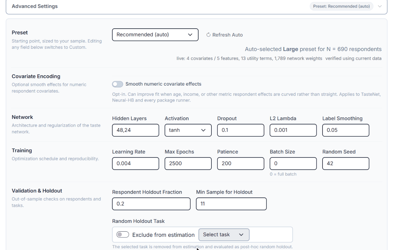
Figure 3. Advanced Settings of the Pizza run. For 690 respondents the auto preset chose Large: hidden layers 48,24, learning rate 0.004, 2,500 epochs.
The panel is grouped into Preset (with Refresh Auto and a live line counting covariates, features, utility terms and network weights), Covariate Encoding (Smooth numeric covariate effects), Network, Training and Validation & Holdout. Editing any field switches the preset to Custom.
Every setting is documented below. The Default column shows the plain defaults; the auto preset replaces several of them depending on your sample size, as Figure 3 shows.
Setting
Default
Description
Preset
Recommended (auto)
Auto-selects architecture based on sample size. Options: Recommended (auto), Small Study (< 200), Medium Study (200-499), Large Study (500-1499), Very Large Study (>= 1500), Custom. The Refresh Auto button next to the selector switches back to Recommended (auto) and recalculates from the current covariates and model setup
Hidden Layers
32, 16
Network architecture. “32, 16” = two hidden layers with 32 and 16 neurons
Activation
tanh
Activation function: tanh (default) or elu
Dropout
0.10
Fraction of hidden units randomly zeroed during training (regularization)
L2 Lambda
0.001
Weight decay penalty to prevent overfitting
Label Smoothing
0.05
Softens 0/1 choice targets to prevent overconfident predictions
Learning Rate
0.005
Step size for the Adam optimizer
Max Epochs
2000
Maximum training iterations. In-app: up to 5,000 for standard TasteNet, up to 10,000 with Neural-HB. Create Package: up to 50,000
Patience
200
Early stopping: stop after this many epochs without validation improvement
Batch Size
0 (full batch)
0 = use all data each step; >0 = mini-batch gradient descent
Random Seed
42
Random seed for reproducibility
Respondent Holdout Fraction
0.20
Share of respondents held out completely for reporting (Validation Split (Report) card, Respondent-Holdout RLH). This split is never used for early stopping or restart selection.
Min Sample for Holdout
11
The respondent holdout is only created when at least this many eligible respondents are available; below that the run trains on everyone and reports no respondent holdout.
Random Holdout Task
Off
Switch Exclude from estimation plus a task dropdown ("Task N"); only shown when the design has random tasks. The selected task is removed from estimation and evaluated as post-hoc random holdout
The auto preset sets these values by sample size:
Preset
Hidden Layers
Dropout
L2 Lambda
Learning Rate
Max Epochs
Patience
Restarts
Label Smoothing
Small Study (< 200)
16,8
0
0.008
0.008
2,000
250
8
0.08
Medium Study (200-499)
32,16
0.10
0.002
0.005
2,000
200
5
0.05
Large Study (500-1499)
48,24
0.10
0.001
0.004
2,500
200
8
0.05
Very Large Study (>= 1500)
64,32
0.10
0.0005
0.003
1,500
120
4
0.03
The recommended preset can raise L2 further when the model has many parameters for the sample. Ranges: 1 to 8 hidden layers with up to 4,096 units, Dropout 0 to 0.9, Label Smoothing 0 to 0.5, Respondent Holdout Fraction 0 to 0.5, Patience at least 10 (In-App Neural-HB at most 800), Max Epochs at least 50.
When to use custom settings
For most studies, the Recommended preset works well. Only switch to Custom if you have a specific reason: very large samples (>2000) may benefit from deeper networks; very small samples (<200) should use smaller architectures with higher dropout.
Neural-HB settings
When the Neural-HB switch is on, a small panel with two additional fields appears directly under the options bar. Both are pre-filled by the auto preset based on your sample size and model complexity; the suggested values are solid defaults and rarely need manual tuning.
Setting
Auto suggestion
Description
delta L2 per task
about 1.7 at N = 50 down to about 0.8 at N = 5,000, decreasing with sample size
Weight of the shrinkage prior on the individual deviations δi relative to the choice likelihood. 1.0 is the neutral Bayesian weighting. Lower values (0.6 to 0.9) let individuals move further away from the neural mean: better fit, higher overfitting risk. Higher values (1.1 to 1.6) keep utilities closer to what the profile predicts. Values above roughly 2 effectively switch individual deviations off (the result collapses toward plain TasteNet), and 0 removes shrinkage entirely (heavy overfitting). The quick-set chips under the field (0.6 / 0.8 / 1.0 / 1.3 / 1.6) mark the sensible grid; a good robustness check is to rerun with 0.6 and 1.6 and confirm your conclusions hold.
Final refit epochs
about 220 to 400, increasing with sample size
After the best restart is selected, the winning model is refit for this many extra epochs on the training tasks plus the internal selection tasks, with hyperparameters frozen. The report task holdout stays excluded, and the reported holdout metrics are re-evaluated on the refit model. More epochs stabilize the final utilities; excessive values can overfit. 0 skips the refit. In-app runs allow up to 1,000 epochs; Create Package allows up to 5,000.
With Neural-HB on, Advanced Settings also shows a Forecast Diagnostics rail with three optional, experimental checks (posterior-based restart selection with a draws-per-restart field, a top-3 new-respondent prediction comparison, and an independent new-respondent calibration). Their results appear only in the Technical Diagnostics workbook. The Smooth numeric covariate effects switch (off by default) has its own row, Covariate Encoding, and is available with and without Neural-HB.
3.7 Running
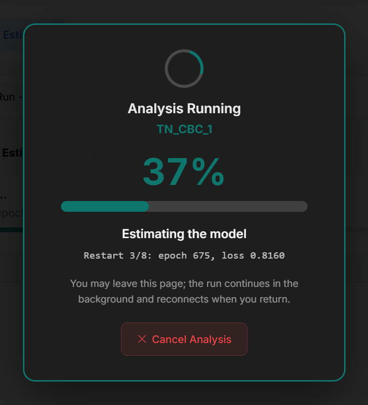
Click Run. A full-screen panel Analysis Running shows the run name, the percentage, the current step (for example "Preparing respondent covariates", then "Estimating the model") and a detail line with the current restart, epoch and loss. You may leave the page; the run continues and the page reconnects when you return.
Figure 4. The Pizza run during training. The whole Pizza run (8 restarts of up to 2,500 epochs plus Fast SHAP) took about 3 minutes.
Cancel Analysis stops the run at any time. When training is complete, Choicery switches to the Results step.
In Create Package mode the Run button does not train anything. It first creates an external run, then generates and downloads the package ZIP, and finally reloads the estimation view with the new run selected and waiting for an import.
4. Interpreting Results
TasteNet results go beyond standard utility estimates. The key differentiator is the SHAP-based covariate analysis, which explains not just what preferences look like but why they differ across respondents. The figures below come from the Pizza run TN_CBC_1 (690 respondents, covariates food_involvement_z, lay_rationalism_z, age, gender, Recommended preset). The Results header has a Download PDF button for the whole page.
From top to bottom the page shows: the meta bar, Covariate Importances, Attribute Importances, Preference Curves by Covariate, Individual Covariate Contributions and the Beeswarm Plot (both collapsed, click Expand), Group Comparison, Covariate Group Comparison, Group Utilities / Coefficients and Summary Utilities / Coefficients (collapsed, with CSV), Holdout Validation, Probability Calibration and Covariate Interactions (collapsed), and Model Diagnostics & Fit Metrics.
4.1 Meta Bar and Model Diagnostics
The top of the results page shows a slim meta bar, laid out like the Preference Analysis (HB) results page: identity first, the headline quality numbers after it. Every label carries a tooltip with the exact definition.
Figure 5. Meta bar of the Pizza run. The respondent holdout scores 0.480 against a chance level of 0.250, so the four covariates carry real information about preferences.
N: Respondents included in the estimation after covariate missing-value policy and data filtering.
Estimation: TasteNet comes first (also for Neural-HB runs).
Estimation tasks: Original survey tasks used in estimation. Best-Worst and dual-response stages are modeled as separate choice observations internally, but all stages from one survey task count as one task here (13 BW-CBC tasks are displayed as 13 tasks, not 26).
Active Run: the run whose results you are looking at.
All-Observed RLH (Point): with a "Chance ... · Lift ...x" line. Root Likelihood across every respondent in the result file. It can mix fitted respondents and report-holdout respondents, so it is a descriptive score, neither a pure training nor a pure holdout metric. Always optimistic.
Respondent-Holdout RLH (Point Mean): held-out people scored with the covariate prediction only. For a plain TasteNet run this is the mean network; for a Neural-HB run it is the final exported Neural-HB mean network without any individual delta. This is the headline validation number in both cases. Runs estimated before the current release show the value of a separately trained mean-only benchmark instead; the tooltip says so.
The two task-holdout variants of Neural-HB runs (posterior-predictive and point) are not in the meta bar; they live in Model Diagnostics & Fit Metrics (below).
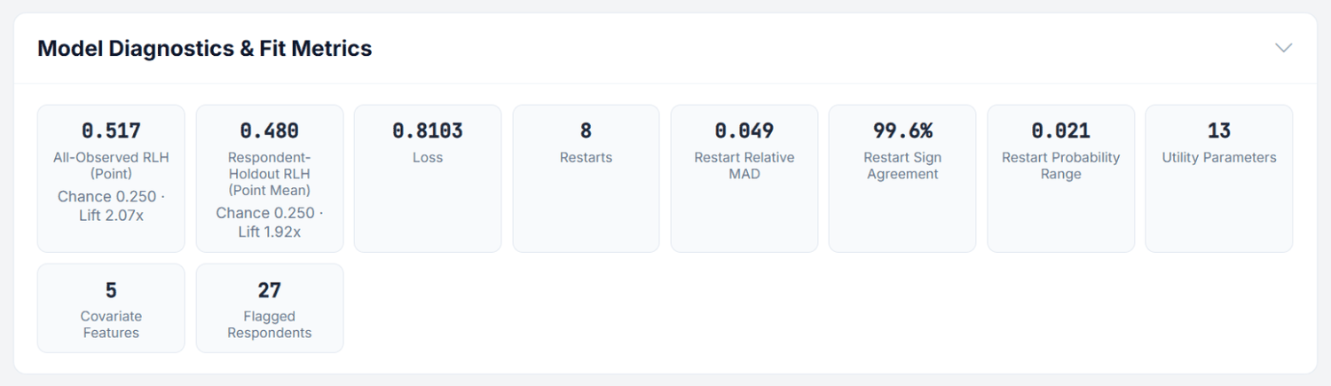
Figure 6. Model Diagnostics & Fit Metrics (opened). The 8 restarts agree closely: 99.6% of the utility signs match.
Everything else lives at the bottom of the page in Model Diagnostics & Fit Metrics, a collapsible section in the same style as on the HB results page. It holds the full metric set as cards: All-Observed RLH (Point), Fitted-Task RLH (Point), Task-Holdout RLH (Posterior-Predictive), Task-Holdout RLH (Point), Respondent-Holdout RLH (Point Mean), Loss, the Best/Worst and None follow-up stage splits (BW-CBC, DR-CBC), Restarts plus three descriptive restart-stability cards (Restart Relative MAD, Restart Sign Agreement, Restart Probability Range), Utility Parameters, Covariate Features, and the number of Flagged Respondents. Each RLH card shows its chance RLH and lift as a second line, and every card has a tooltip explaining exactly what it measures.
The RLH metrics at a glance
TasteNet and Neural-HB report several RLH variants because they validate different things. This table is the map:
Metric
Where
What it measures
Comparison to HB
All-Observed RLH
Meta bar, Model Diagnostics
Geometric mean of predicted probabilities for the chosen alternatives across every respondent in the result file; mixes fitted and report-holdout respondents
Closest to HB’s Mean RLH, but optimistic in both worlds; do not use it to pick a winner
Fitted-Task RLH
Model Diagnostics
RLH of the final exported model on exactly the tasks it was fitted on
The clean in-sample number when you need one; still optimistic
Respondent-Holdout RLH (Point Mean)
Meta bar, Model Diagnostics
Held-out people, scored with the covariate prediction NN(z) only (for Neural-HB the final exported mean network without deltas); no individual choice data used
HB has no counterpart unless the HB run enabled its optional respondent holdout; measures covariate portability, HB’s numbers do not
Held-out tasks of observed respondents; probabilities averaged over per-respondent delta posterior draws
The closest analogue to an HB posterior-predictive score, but not the same statistic: Choicery’s HB fitted RLH averages draw-wise RLHs, whereas this number averages the choice probabilities over delta draws first. Compare it only with another posterior-predictive score on the same tasks and weights
Task-Holdout RLH (Point) (Neural-HB)
Model Diagnostics
Same held-out tasks, but scored with posterior-mean utilities only
Ignores posterior uncertainty, so it is systematically less comparable to HB; usually slightly lower than the posterior-predictive value
Chance RLH
Model Diagnostics, Holdout Validation cards
Random-choice baseline, 1/J weighted by the valid alternatives per scored observation
Same definition in HB; any model RLH must clearly beat it
MHP (Mean Hit Probability)
Holdout Validation cards
Average predicted probability of the actually chosen alternative
Same concept as HB’s MHP; unlike hit rate it rewards confident correct predictions
Hit Rate / Ratio
Holdout Validation cards
Share of observations where the highest-probability alternative equals the observed choice; Ratio = hit rate divided by chance
Same concept as HB’s holdout hit rate; a ratio of 2x means twice as accurate as guessing
Best/Worst splits (BW-CBC only)
Model Diagnostics, Holdout Task Breakdown
The same metrics reported separately for the Best stage and the Worst stage of each task
Worst-stage scores are typically lower in every estimator; compare stage against stage, never Best against Worst
Why Neural-HB has two validation notions
Neural-HB has two jobs. The neural mean fθ(z) should generalize from covariates to new respondents; the MAP deviation δn should recover additional signal for observed respondents with choice histories. Respondent-holdout RLH tests the first job. Task-holdout RLH tests the second. A high train RLH alone is not enough, because it can simply mean that the respondent deviations fit the observed tasks well.
What is a good RLH?
For a 3-alternative CBC, chance RLH = 0.333 (= 1/J). A Respondent-Holdout RLH of 0.55-0.70 is typical for covariate-driven models on realistic samples; 0.70+ indicates strongly informative covariates. If it is within about 3 percentage points of chance, the covariates are not predictive enough, add attitudinal items or switch to HB (where each respondent’s own choices refine their utility). Note: TasteNet’s Respondent-Holdout RLH is not directly comparable to HB’s RLH, because HB has already used each respondent’s own choices while TasteNet has not (Section 15.2).
4.2 Covariate Importances
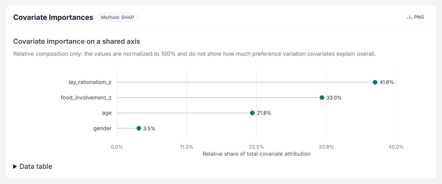
Figure 7. Covariate Importances of the Pizza run. Gender, which plays no role in the data, ends clearly last.
This is TasteNet’s signature output. A dot plot titled "Covariate importance on a shared axis" ranks which covariates most influence preferences overall; the values add up to 100% and show the composition, not how much of the preference variation the covariates explain. Data table opens the numbers. A small Method tag next to the heading states how the numbers were produced: Method: SHAP, Method: Mean-Net SHAP for Expected-Gradient SHAP on a Neural-HB mean network, Method: Gradient × SD for the fast sensitivity proxy, Method: Weight heuristic for the connection-weight fallback when SHAP is unavailable (the Excel sheet labels it “Weight-based (fallback)”), which is explicitly not SHAP, and Method: Not available when no attribution values could be computed. The Fast and Full distinction (Method: SHAP · Fast, Method: SHAP · Full) is shown on the Individual Covariate Contributions section instead, see 4.5.
SHAP (SHapley Additive exPlanations) decomposes each respondent’s predicted utility into additive contributions from each covariate. The importance score reflects the average magnitude of SHAP values across all respondents and all utility parameters.
In Hybrid and Neural-HB package runs, SHAP still explains the neural mean, not the respondent-specific residual or MAP deviation. This is intentional: SHAP is a covariate attribution method, and the respondent-specific component is learned from choice history rather than from covariates. Therefore, SHAP answers “which covariates drive the neural prior mean?”, while the final utilities used for observed-respondent simulations may also include respondent-level refinement.
Example Reading
If the SHAP importance chart shows Age: 46%, Tech Affinity: 41%, Gender: 13% (importances are normalized to sum to 100%), this means that Age and Tech Affinity are the two strongest drivers of preference heterogeneity, while Gender plays a relatively minor role in explaining why people’s conjoint preferences differ.
4.3 Attribute Importances
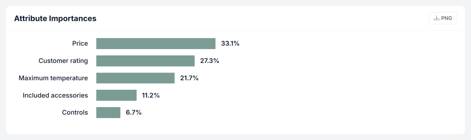
Figure 8. Attribute Importances of the Pizza run, almost identical to the HB run (32.9 / 26.6 / 22.0 / 11.2 / 7.3%).
This chart shows the relative importance of each conjoint attribute in driving choice decisions, the same concept as in HB estimation. With product interactions the heading reads Main-Effect Attribute Importances. Attributes are displayed as horizontal bars, sorted in descending order of importance. When a package run produced bootstrap confidence intervals, the heading reads Attribute Importances (Bootstrap CI) and a small table with CI 95% Low and CI 95% High is appended underneath the bars.
This answers: “Which attributes matter most for the choice?” (as opposed to the covariate charts, which answer “Which covariates drive preference heterogeneity?”).
For MaxDiff and Anchored MaxDiff runs the same section shows the item preference metric instead, labelled with the run’s own metric name, and reports a normalized fixed-competitor win index rather than an attribute importance.
4.4 Preference Curves by Covariate
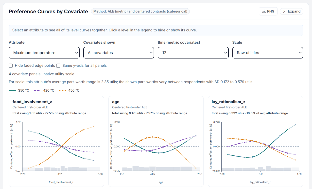
This section plots the fitted systematic TasteNet function directly: for the selected attribute, it shows how every one of its part-worths changes across the range of each respondent covariate. It is not SHAP, not a choice probability and not a market share. The method tag reads Method: ALE (metric) and centered contrasts (categorical).
Metric covariates are rendered as centered first-order ALE curves over the observed covariate distribution, one point per equal-count bin.
Categorical covariates are rendered as unconnected, observed-share-centered point contrasts (grouped lollipops), because their levels have no order. Centering means that even the reference category is not required to sit at zero.
Support bars in grey count the model inputs per bin after imputation. Thin bins and metric tail bins outside the central 90% of observed values are drawn faded.
No confidence bands. Estimation uncertainty is not calculated for these curves.
Figure 9. Preference Curves for Maximum temperature. With rising food involvement the utility of 450 °C climbs (total swing 1.83 utils, 77.5% of the attribute range), age moves it little (7.6%).
The controls above the panels are:
Attribute: all level curves of one attribute are shown together. Click a level in the legend to hide or show its curve.
Covariates shown:All covariates or a single one. Panels exist per covariate and bin count, not per attribute level.
Bins (metric covariates): 6, 8, 12 (default), 16 or 20 equal-count bins. Tied values can collapse bins below the chosen number.
Scale:Raw utilities, Zero-centered diffs (each respondent contributes on their own zero-centering factor; older runs use the population-average fallback named in the footnote) or % of attribute range, where 100% equals that attribute’s average part-worth range.
Hide faded edge points: trims the faded points at the left and right end of each curve. Faded points in the middle stay visible.
Under the panels, a For scale line puts the curve magnitudes into perspective: it compares the largest level movement against the attribute’s average part-worth range and against how much the shown part-worths vary between respondents (their SD).
Curves are precomputed, so this view is fast
Since July 2026 the curve panels are calculated once when the run finishes and stored with the run as Covariate_Curves.json, one panel per (bin count, covariate) combination. Opening the Results step therefore only reads JSON; it no longer has to load the neural framework to re-evaluate the model. Older runs and unusually wide studies that exceed the stored panel budget fall back to live computation, which is slower but produces the same numbers.
4.5 Individual Covariate Contributions
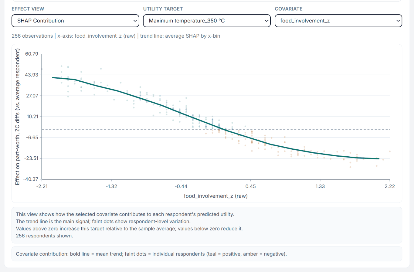
The most detailed view into covariate-preference relationships, one dot per respondent. Select an Effect View, a Utility Target (a specific attribute level, or Importance Target for MaxDiff) and a Covariate to see how that covariate influences preferences for that level. A short reading guide above the chart explains the encoding: each dot is one respondent, points above the yellow zero line push the preference above the sample average, points below push it down, and the orange dot marks where the fitted trend crosses zero. It states the result in words before you read the plot.
Figure 10. Individual Covariate Contributions: the more someone cares about food, the less they value an oven that only reaches 350 °C. Each dot is one of the 256 respondents shown.
The section is collapsed by default (click Expand). In-App runs use Fast SHAP on up to 256 respondents; a yellow note says so and points to the package for full SHAP. Derived reference levels, marked (derived) in the Utility Target list, have no SHAP values of their own: Choicery rebuilds them as the negated sum of the estimated levels of the same attribute. For the nonlinear network this is an approximation, and the chart says so; read it as directional.
Three Effect View modes are available (the first is renamed to Mean-Net SHAP Contribution or Gradient x SD Contribution when another method was used):
View Mode
What It Shows
Best For
SHAP Contribution
Raw SHAP value vs. covariate value. Shows the direct contribution of this covariate to the predicted utility.
Understanding the functional form of the covariate effect
Predicted Utility by Observed Group
Group mean utilities using covariate groups. Shows how groups differ in their predicted preference for this level.
Comparing demographic groups
Predicted Utility by Isolated Covariate Change
Counterfactual “what-if” analysis. Varies only the selected covariate and keeps every respondent’s other covariates as they are (partial dependence).
Isolating the causal-direction effect of a single covariate
For numeric covariates, the chart shows a scatter plot with a trend line. For categorical covariates, it shows a jitter plot with group means and 95% ranges.
A note on scale: the displayed values are on each respondent’s zero-centered utility scale, so the decomposition is exact within a respondent, but cross-respondent trends combine the covariate effect with differences in per-respondent scaling. For MaxDiff runs the utilities are shown on their native logit scale instead.
Two smaller panels appear underneath when they apply: Binary Group Difference (A - B, 95% CI of mean difference) for two-group covariates, and Effect of each level vs reference for multi-level categorical covariates.
4.6 Beeswarm Plot
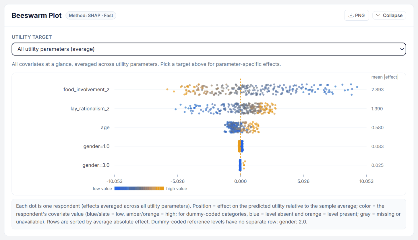
Figure 11. Beeswarm Plot (expanded). Food involvement spreads the predicted utilities most; the gender rows stay close to zero. Dummy-coded categories show one row per category except the reference.
Collapsed by default. A beeswarm chart that puts all covariates on one screen, sorted by average absolute effect on the selected target. Each dot is one respondent; its horizontal position is the covariate’s contribution and its colour encodes the respondent’s own value of that covariate (blue for low, amber for high). The single control, Utility Target, defaults to All utility parameters (average).
Use this as the entry point (which covariates matter at all, and does a high value push utility up or down?), then drill into one covariate with the Individual Covariate Contributions chart or the preference curves.
4.7 Group Comparison
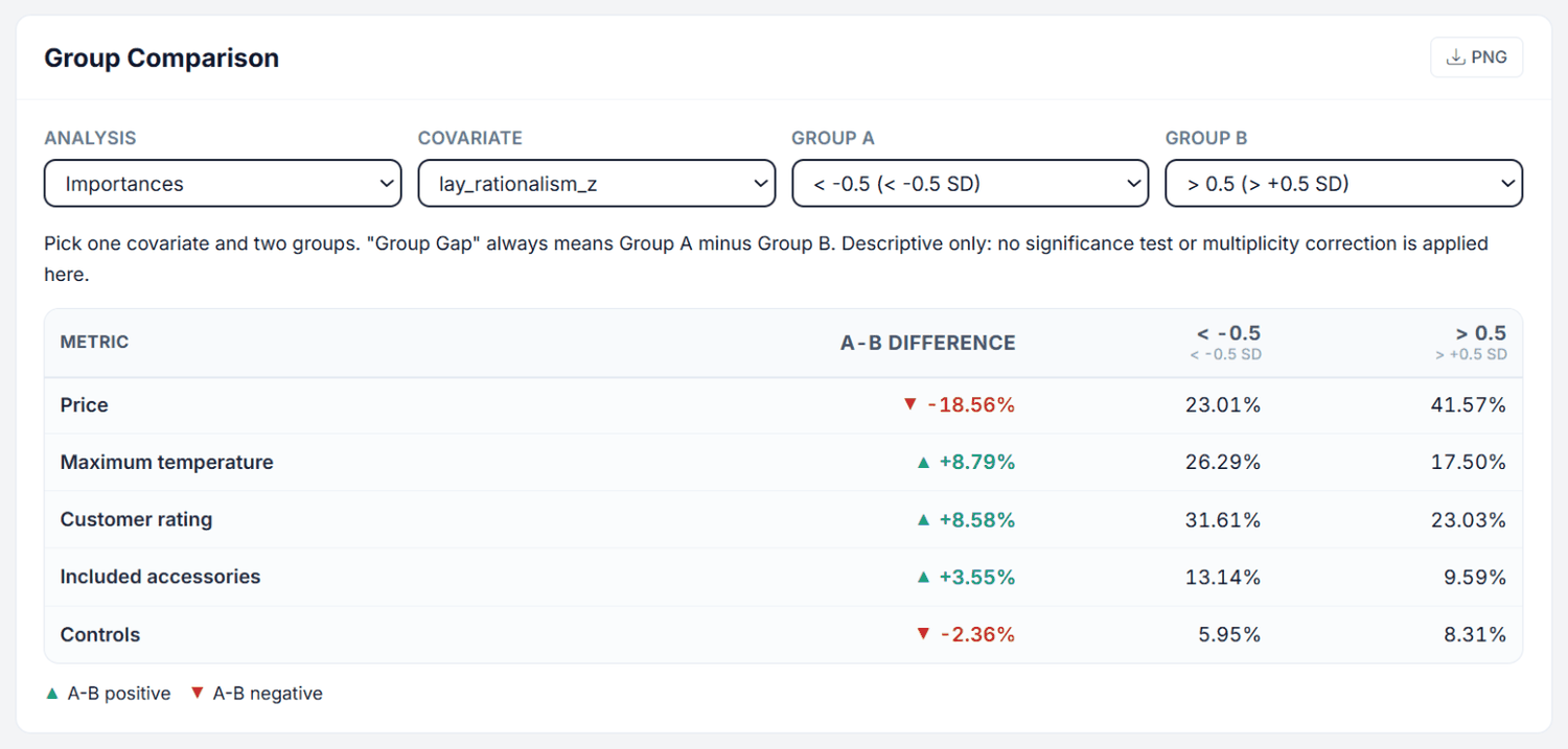
Compare how two respondent groups differ in their preferences. This is often the most actionable output for marketing teams. Pick one Covariate and two groups (Group A, Group B); the chart always reports the gap as Group A minus Group B, with each group’s own mean shown alongside it. An Attribute Filter narrows the chart to a single attribute where that makes sense.
Figure 12. Group Comparison: respondents with high lay rationalism give price 41.6% of the importance, those with low lay rationalism 23.0%.
Four Analysis modes:
Importances: Relative attribute importance for each group.
Level Utilities: Side-by-side part-worth utilities for each attribute level. For MaxDiff runs this option is labelled Fixed-Competitor Win Index instead.
Attribute Strength (max-min): The overall range (max − min utility) within each attribute, per group.
Within-Attribute Level Gap: The difference between groups for each specific level.
All group gaps are descriptive: no significance test or multiplicity correction is applied. The Group Differences sheet of the results workbook adds Cohen’s d as an effect size.
Example Reading
Comparing < 36.9 (< -0.5 SD) against > 51.2 (> +0.5 SD) on Age in Attribute Strength mode might reveal that younger consumers weight Design 3x more than older consumers, while older consumers weight Brand Trust 2x more. This directly informs age-targeted product positioning.
Covariate Group Comparison and the utility tables
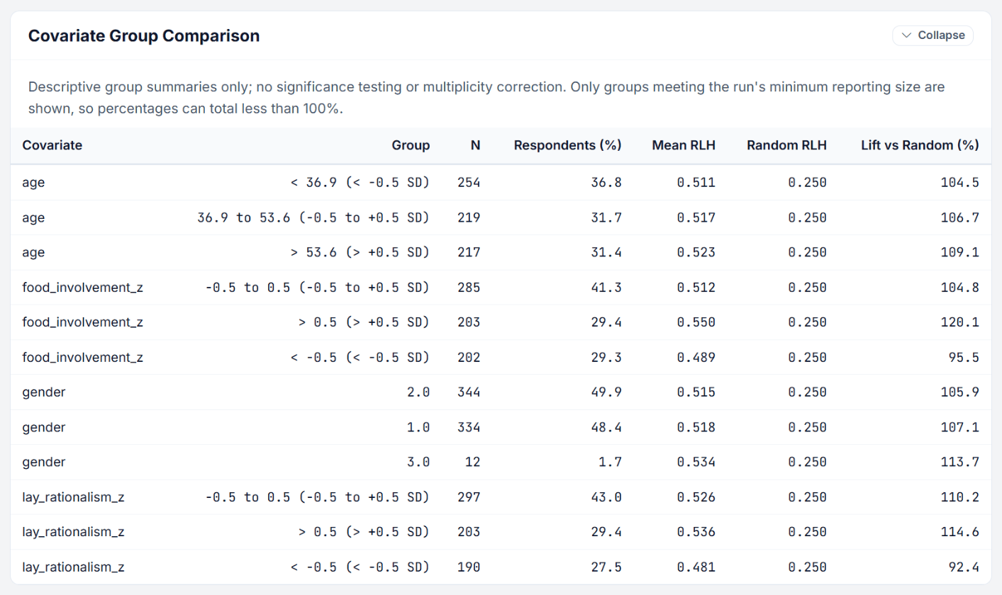
Covariate Group Comparison (open by default) lists every derived group with its size and fit: N, Respondents (%), Mean RLH, Random RLH and Lift vs Random (%). It shows for whom the model predicts well. Only groups meeting the minimum reporting size appear, so percentages can add up to less than 100%. Below it, Group Utilities / Coefficients and Summary Utilities / Coefficients (both collapsed, with a CSV button) list the utilities per group and for the whole sample.
Figure 13. Covariate Group Comparison of the Pizza run. Categories appear with their stored codes (gender 1.0, 2.0, 3.0).
Covariate Interactions and Probability Calibration
Both sections come after Holdout Validation and are collapsed by default (Probability Calibration first, tagged "Top-label reliability"; Covariate Interactions second, tagged "Learned pair effects").
Covariate Interactions ranks covariate pairs by how much they change each other’s effect on predicted utilities. The strongest pair scores 100; the ratio column relates the interaction to the two separate effects, and the last column names the attribute it affects most. It is a model non-additivity diagnostic, not a significance test.
Probability Calibration shows a top-label reliability diagram of the model’s largest predicted probability against the observed hit rate, with the expected calibration error, a multiclass Brier score and a resampled reference band (drawn only with at least 30 respondents in the split).
Two smaller controls are easy to miss: the Preference Curves card has a Same y-axis for all panels checkbox (off by default) so effect sizes can be compared across covariates, and the isolated-change view of Individual Covariate Contributions has an ICE View selector (Level, Centered change, Derivative) that adds thin lines for up to 40 sampled respondents on a 21-point grid, showing whether the direction of the effect is shared or heterogeneous.
4.8 Neural-HB: Covariates vs Individual Residuals
This section appears only for Neural-HB runs. It splits the modeled utility heterogeneity into two bars per utility parameter: Covariates, the share explained by the neural mean NN(z), and Individual residual, the share carried by the respondent-specific posterior-mean deviations. Headline numbers report the mean and median covariate-explained share, and a per-attribute breakdown is available below the chart.
Read it as a diagnosis of your covariate set: a high covariate share means the profile variables really do explain preference, a high residual share means most of the differences between people are individual taste that your covariates do not capture. The heading tooltip states that the deltas are trained with a variational objective, not with MCMC.
4.9 Holdout Validation
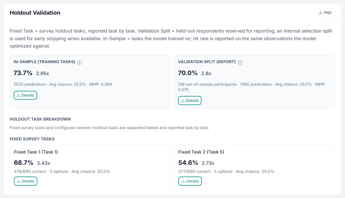
Figure 14. Holdout Validation of the Pizza run. The fixed tasks are predicted about as well as with HB (68.7% vs 67.8% and 54.6% vs 52.5%), although TasteNet uses no individual choices.
The Holdout Validation section reports predictive accuracy on up to three levels, each as a card. A card reads like this: the big percentage is the hit rate (share of observations where the model’s highest-probability alternative matches the observed choice), the x-value next to it is the lift over guessing (hit rate divided by average chance), and the small line underneath gives the number of scored predictions, the average chance rate (weighted by the valid alternatives per observation, so it is not always exactly 1/J), and the MHP (mean predicted probability of the chosen alternative). Every card has a Details button that downloads the per-observation prediction CSV behind the number.
In-Sample (Training Tasks): accuracy on the tasks the model trained on. Optimistically biased, useful only as a ceiling. Example: 88.7% with 2.66x lift means near-ceiling in-sample fit.
Validation Split (Report): accuracy on held-out respondents reserved for reporting (an internal selection split handles early stopping, so this number stays honest). For plain TasteNet this is the primary quality metric; a Primary badge marks whichever card the run treats as its main reporting metric.
Holdout Task Breakdown: split into Fixed survey tasks and Configured random-holdout tasks. If the design contains fixed holdout tasks, each one gets its own card, scored only task by task. These tasks were never part of training, making this the most stringent test.
Best and Worst cards (BW-CBC)
For Best-Worst CBC, every fixed holdout task appears as two cards, one for the Best answer and one for the Worst answer, for example “Task 5 - Best: 69.7%, 2.09x” and “Task 5 - Worst: 61.7%, 1.85x”, plus an “Exact Best-Worst Pair” card when the run reports it. Both stages share the same chance rate (same number of alternatives), but their hit rates can differ in either direction: in the Pizza study the Worst answer was easier to predict than the Best (HB run: 61.4 against 53.6 percent in fixed task 1). Compare Best against Best and Worst against Worst, for example against the corresponding cards of an HB run, and do not read a Best-vs-Worst gap as a model problem.
5. Exporting Results
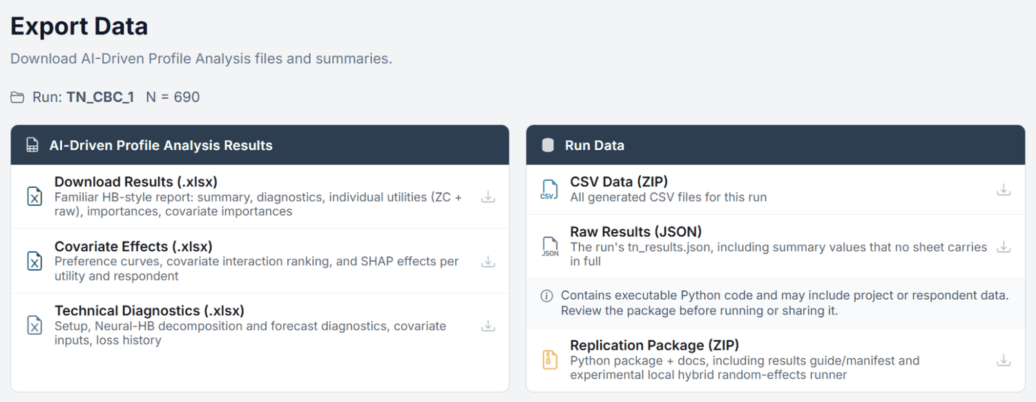
Step 3 of the strip, Export, opens Export Data with two cards. AI-Driven Profile Analysis Results holds three Excel workbooks; Run Data holds the raw files and the replication package.
Figure 15. The Export step of the Pizza run.
Three disjoint workbooks, no duplication
As of July 2026 the three Excel files deliberately do not overlap. Everything you report lives in Results, everything about covariate effects lives in Covariate Effects, and Technical Diagnostics is a supplement that repeats neither. Technical Diagnostics used to be a superset of Results; it is not any more, so download all three if you want the complete picture.
Download
Contents
Audience
Download Results (.xlsx)
The presentation workbook, laid out like the HB report (see 5.1). File name TasteNet_Results_<run>.xlsx
Everyone; this is what you share
Covariate Effects (.xlsx)
Preference curves for every attribute and covariate on all three scales, plus SHAP per utility, per respondent and signed per contribution (see 5.2). File name TasteNet_Covariate_Effects_<run>.xlsx
Anyone answering “which profile drives which preference?”
Technical Diagnostics (.xlsx)
Setup, Neural-HB decomposition and diagnostics, covariate inputs, loss history (see 5.3). File name TasteNet_Technical_<run>.xlsx
Analysts auditing the model, reviewers
CSV Data (ZIP)
Every generated CSV file of the run, including machine-readable results and holdout prediction files. File name TasteNet_Data_<run>.zip
Further analysis in R / Python / SPSS
Raw Results (JSON)
The run’s tn_results.json, including summary values that no sheet carries in full. File name tastenet_results_<run id>.json
Scripted post-processing, debugging
Replication Package (ZIP)
Self-contained Python package for an independent local rerun, with docs, manifest, and optional bootstrap confidence intervals. It contains executable code and may include project or respondent data, so review it before running or sharing it
Independent verification, method audits
5.1 The Results workbook, sheet by sheet
If you know Choicery’s HB report, you already know the first six sheets: same names, same order, same conventions. The TasteNet-specific sheets follow after them.
Sheet
What it contains
When you need it
Summary
Mean zero-centered utility per level with SD and attribute importance, like the first sheet of the HB report
First stop; the table you paste into a presentation
Settings & Diagnostics
Run information, sample, model quality (RLH vs. chance), holdout validation
Documenting methodology; checking run quality before using results
Individual Utilities ZC
One row per respondent, zero-centered diff utilities (HB convention)
Segmentations, external simulators, any per-person analysis on the comparable ZC scale
Individual Raw
One row per respondent, raw logit-scale utilities; linear attributes on the per-unit scale
Custom choice-probability calculations where the raw scale matters
With a respondent holdout the workbook adds a Validation Split (Report) sheet.
For Neural-HB runs the individual utility sheets contain the total utilities (neural mean plus individual delta), so they are directly comparable to an HB export. Anchored MaxDiff runs additionally include Purchase Probability, Anchored Utilities, Consideration Sets, and Anchor Summary sheets.
5.2 The Covariate Effects workbook
This workbook answers the one question TasteNet exists for: how do respondent characteristics shift the estimated part-worths? It contains the preference-curve data behind the chart in 4.4, the covariate attribution values, and the covariate interaction ranking behind the Covariate Interactions panel. Every sheet is a plain rectangle sharing an Attribute / Level / Covariate vocabulary, so sheets can be pasted side by side into one table.
Sheet
What it contains
When you need it
Read Me
What is and is not in this file, one line per sheet, and how to read each effect column
First stop, especially before sharing the file with someone else
Preference Curves
One row per attribute, level, covariate and bin, with bin edges, respondent count, a Low Support marker, and the effect on all three scales: Effect (utils), Effect (ZC diffs), Effect (% of avg range)
Rebuilding the curves in your own tool; exact numbers behind the chart
Curve Method
One row per covariate: method (centered first-order ALE or observed-share-centered discrete contrast / partial dependence), coding, reference category, how many bins or categories it actually got, respondents, low-support threshold
One row per attribute with its average part-worth range and the min and max level SD, plus the population factor used only as a scale reference; exact curves use each respondent’s own factor
Judging whether a curve movement is large or small
SHAP by Utility
One row per utility parameter and covariate: mean absolute SHAP and its share
Ranking covariates per attribute level
SHAP Values
One row per respondent, mean absolute SHAP per covariate feature
Respondent-level attribution analysis
SHAP Beeswarm
Long format, one row per respondent, utility parameter and covariate, with the signed SHAP value and both the encoded and the raw feature value
Rebuilding the beeswarm chart or running your own attribution statistics
Covariate Interactions
One row per covariate pair: relative strength (top pair = 100), interaction to separate-effects ratio, interaction RMS in utils, strongest affected attribute
Judging whether two profile variables change each other’s effect
Three scale columns, three different meanings
Effect (utils) is the shift of that part-worth against the sample average on the native utility scale, not the part-worth itself. Effect (ZC diffs) accumulates each respondent with that respondent’s own zero-centering factor; older runs without exact curves use a population-average fallback and say so in the workbook. Effect (% of avg range) expresses the effect as a share of that attribute’s average part-worth range and is empty for linear attributes, which have no level range. None of the three carries a confidence interval: these are model associations, not causal effects.
The SHAP Beeswarm sheet is capped at Excel’s own row limit. If the run exceeds it, the Read Me sheet says so and points to the complete file in the run folder.
5.3 The Technical Diagnostics workbook
Technical Diagnostics is a supplement. It repeats nothing from Results and nothing from Covariate Effects. Sheets appear only when the run produced them: Neural-HB sheets only for Neural-HB runs, hybrid sheets only for legacy hybrid packages, and so on.
Group
Sheets
What they are for
Setup & training
Setup, Loss History
Every hyperparameter with its impact on results; per-epoch training and validation curves for overfitting checks
Covariate internals
Covariate Groups Overview, Group Attr Importance, Covariate Values, Covariate Features
Group compositions, per-group importances, and exactly which covariate encodings the network saw
Neural-HB deep dive
Neural-HB Codebook, Overview, Decomposition, Residuals, Prior Mean, Delta, Sigma, Scales, Task Holdout, Resp Holdout, Cold Comparison, Cold Predictions, Restarts, Forecasts (only when a Forecast Diagnostics option was enabled); plain TasteNet runs get a TasteNet Restarts sheet instead
The complete Neural-HB decomposition and diagnostics; see the reading guide below
Legacy hybrid
Hybrid Mean Utilities, Hybrid RE Residual, Hybrid Final Utilities, Hybrid Latent Factors, Hybrid Factor Loadings, Hybrid Respondent Diagnostics
Only for imported Hybrid Random Effects packages (Section 12)
Reading the Neural-HB sheets
Neural-HB Codebook: definitions of every field used in the other Neural-HB sheets. Read this first.
Neural-HB Overview: the run’s key numbers in one place: All-Observed RLH, Fitted-Task RLH, both task-holdout variants, the Cold-Start Benchmark RLH, chance RLH, delta L2 per task, the final tau, and how much heterogeneity the covariates explain. The Task-Holdout RLH (Posterior-Predictive) row is the HB-style draw-averaged number to use when comparing against an HB run.
Neural-HB Decomposition: per utility parameter, how much of the cross-respondent variance the neural covariate component NN(zi) explains versus the individual deltas. High covariate share = profile-driven preference; high residual share = individual taste your profiles do not capture.
Neural-HB Residuals: per-utility spread of the deltas (sigma, mean absolute delta): where individuals deviate most from their profile prediction.
Neural-HB Prior Mean / Delta: per-respondent matrices of the two utility components that make up the exported total utilities.
Neural-HB Sigma / Scales: the learned prior scale per parameter, and per-respondent scale factors (choice consistency).
Neural-HB Task Holdout / Resp Holdout: the per-observation holdout predictions behind the reported RLH numbers.
Neural-HB Restarts: the score of every random restart and which one was selected.
5.4 Which download when?
Presenting or sharing results: Download Results (.xlsx).
“Which respondent characteristics drive which preference?”: Covariate Effects (.xlsx).
Method questions, reviewer pushback, “how was this fitted?”: Technical Diagnostics (.xlsx).
Further analysis in R, Python, or SPSS: CSV Data (ZIP), or Raw Results (JSON) for the summary values no sheet carries in full.
Choicery supports three respondent-level estimators: HB (hierarchical Bayes), LC (latent class), and TasteNet. Each answers a different substantive question. The Concomitant-HB variant, HB with linear covariate effects on the population mean, is available as an optional upper layer on top of any HB run via the Create-Package covariate panel (see HB tutorial). Aggregate MNL (no heterogeneity at all) is intentionally not offered as a standalone estimator; if you ever need aggregate utilities, a Latent Class run with Min Classes = 1 estimates exactly that model as its one-class solution, and the Interaction Search Excel export contains a full Main Effects (Aggregate MNL) sheet.
Scenario matrix
Scenario
Best Method
Why
Need individual utilities for market simulation
HB
Posterior updating from each respondent’s own choices; no covariates required.
Want to understand WHY preferences differ
TasteNet
SHAP decomposition of the covariate-to-utility mapping. HB offers only the linear ΔTzn layer.
Have rich respondent covariates (attitudes, usage, psychographics)
TasteNet
Learns nonlinear interactions (e.g. “price sensitivity depends on income × household size”) automatically.
Have respondent covariates but need posterior uncertainty
HB + Covariates
Concomitant HB (βn ∼ MVN(ΔTzn, Σ)): covariate layer in mean, individual random effects on top, proper credible intervals per coefficient.
Need discrete, nameable market segments
LC
Joint estimation of segment memberships + segment-specific preferences, better than k-means on HB utilities.
Predict preferences for new respondents with known covariates only
TasteNet
Deterministic βn = fθ(zn), ship the trained network, apply to any new covariate vector. HB needs choice data per person; concomitant HB gives only the linear covariate mean. Powers the Persona tab.
Small sample (<150 respondents)
HB
Bayesian shrinkage handles small N with posterior uncertainty. Neural nets need enough respondents to learn nonlinear mappings.
No covariates collected
HB / LC
TasteNet is unusable without covariates; HB and LC work without them.
Large sample (>1,500) with many attitudinal items
TasteNet
Neural mapping captures nonlinear interactions across many covariates. With ample data, the regularization stack (dropout, L2, label smoothing, early stopping) handles overfitting cleanly.
Need better observed-respondent RLH but want to keep the neural covariate model
Neural-HB MAP
Uses the neural network as a nonlinear prior mean and adds respondent-specific MAP deviations from each person's choice history. Compare task-holdout and respondent-holdout RLH separately.
Sensitive data that cannot leave the analyst’s machine
Create Package
HB and TasteNet both ship as self-contained offline packages (Julia / Python). Re-import the result ZIP when done.
Aggregate MNLno standalone estimator
,
Intentionally not offered as its own analysis. A single β for the whole sample ignores heterogeneity; HB strictly dominates (same logit kernel, degenerates to aggregate in the zero-heterogeneity limit, delivers individual utilities required by every downstream module). If you do need aggregate utilities, two indirect routes exist: a Latent Class run with Min Classes = 1 (the one-class solution is exactly an aggregate MNL) and the Main Effects (Aggregate MNL) sheet in the Interaction Search Excel export.
Complementary, not competing
HB, LC, and TasteNet answer three different questions:
HB: “What does this individual respondent prefer, given all of their choices?”
LC: “How many types of respondents exist, and what are their preferences?”
TasteNet: “How do observed respondent characteristics map into preferences, and how would a new respondent with covariates znew be expected to choose?”
The strongest analysis pipelines run at least two of these and triangulate. HB+TasteNet is a particularly informative pair: HB delivers the point estimates + credible intervals you need for simulation, while TasteNet delivers the covariate-explanation story and the ability to score external personas. Running both and comparing attribute importances and group contrasts often reveals where covariate-driven structure aligns with posterior-driven individual differences (robust findings) versus where they disagree (worth investigating).
They complement each other
TasteNet, HB, and LC are not competitors, they answer different questions. HB: “What does each individual prefer?” LC: “Are there distinct segments?” TasteNet: “Why do preferences differ?” The strongest analysis pipeline runs all three and triangulates findings.
7. Best Practices & Common Pitfalls
Do
Select 5-15 meaningful covariates that you believe could plausibly relate to product preferences. Mix demographics (age, gender, income) with attitudinal items (sustainability attitudes, tech affinity).
Include attitudinal items. They often predict preferences better than demographics alone because they capture the psychological mechanisms behind choice behavior.
Use the auto-recommended preset for network architecture. It has been tuned for typical conjoint sample sizes.
Check Respondent-Holdout RLH. For a standard TasteNet run this is your primary quality metric. It should be well above chance (e.g., >0.50 for a 3-alternative CBC). If it is close to chance, the model is not learning.
Use the covariate charts to tell a story about WHO values WHAT and WHY. This is TasteNet’s unique value proposition, don’t skip it.
Start with In-App mode for exploration; switch to Create Package when you need publication-quality results or the hybrid extension.
Don’t
Don’t run TasteNet without covariates. It collapses to an aggregate MNL model, which is strictly worse than HB.
Don’t include 30+ covariates with <300 respondents. Massive overfitting risk. The neural network will memorize noise instead of learning signal.
Don’t trust results where Respondent-Holdout RLH ≈ Chance RLH. The model is not learning meaningful patterns. Revisit your covariate selection and sample size.
Don’t skip the group comparison charts. They are TasteNet’s key differentiator from HB, this is where the “why” becomes actionable.
Don’t compare TasteNet utilities directly with HB utilities. Different estimation methods produce different scales. Compare relative patterns (e.g., importance rankings), not absolute numbers.
Don’t ignore the restarts count. Use at least 5, ideally 10+ for stable results. With only 1 restart, you may be stuck in a poor local minimum.
The most common mistake
Running TasteNet with only 2-3 demographic covariates on a sample of 100 respondents. This setup cannot work: the neural network has too little information (few covariates) and too little data (few respondents) to learn meaningful covariate-preference relationships. Use HB instead, and add TasteNet when you have richer data.
Part II
Theoretical Background
The methodological foundations of TasteNet-MNL: architecture, training, SHAP, and extensions.
8. Key Definitions
Glossary
TasteNet-MNL
A neural-embedded discrete choice model where taste parameters (part-worth utilities) are learned as functions of respondent covariates via a feedforward neural network. Proposed by Han et al. (2022).
Neural Network (MLP)
A multi-layer perceptron: a feedforward network consisting of an input layer, one or more hidden layers with nonlinear activation functions, and an output layer. Each layer is a linear transformation followed by an element-wise nonlinearity.
Covariates
Respondent-level characteristics used as inputs to the neural network. Examples: age, income, gender, education, attitudinal scale scores, behavioral frequency measures.
SHAP (SHapley Additive exPlanations)
A game-theoretic method for explaining individual predictions by computing the marginal contribution of each input feature. Based on Shapley values from cooperative game theory (Lundberg & Lee, 2017).
Early Stopping
A regularization technique that halts training when the validation loss stops improving. Prevents the model from overfitting to the training data by selecting the epoch with the best generalization performance.
Random Restart
Re-initializing all neural network weights randomly and retraining from scratch. Multiple restarts help avoid poor local minima in the non-convex loss landscape.
Label Smoothing
Replacing hard 0/1 choice targets with softened values: (1−ε) for the chosen and ε/J spread over all valid alternatives (for J = 2 and ε = 0.05 that is 0.025 / 0.975). Prevents the model from becoming overconfident and improves generalization.
Hybrid TasteNet
An extension that adds respondent-level random effects: βi = f(zi) + ui. The residual ui captures unobserved heterogeneity not explained by covariates.
RLH (Root Likelihood)
The geometric mean of predicted probabilities for the chosen alternatives. Computed as exp(LL/N) where LL is the log-likelihood and N is the total number of choice tasks. Higher is better.
Dropout
A regularization technique that randomly sets a fraction of hidden-layer activations to zero during each training step. Forces the network to learn redundant representations, reducing overfitting.
9. The TasteNet-MNL Architecture
9.1 Two-Module Design
TasteNet-MNL consists of two modules that are trained jointly:
Module 1, TasteNet: A feedforward neural network that maps respondent covariates zi to individual taste parameters βi.
Module 2, MNL: A standard multinomial logit model that uses the predicted βi to compute choice probabilities.
The architecture separates taste formation (how covariates shape preferences) from choice generation (how preferences lead to choices). This separation preserves the economic interpretability of the MNL model while allowing the covariate-to-taste mapping to be arbitrarily complex.
9.2 Formal Specification
Following Han et al. (2022), the taste parameter for attribute level k as a function of respondent covariates z is:
where A = activation function (tanh or ELU), T = constraint transform (identity for unconstrained, softplus for sign-constrained parameters),
w(1), w(2) = weight matrices, b = bias vectors, zd = covariate d for respondent n.
For deeper networks (more than one hidden layer), the formula chains multiple layers of the form A(Wz + b) before the final output transformation T.
9.3 End-to-End Training
Both modules are trained jointly via backpropagation on the choice log-likelihood. Gradients flow from the choice probability loss through the MNL module back into the neural network weights. This means the neural network learns to produce taste parameters that best explain observed choices, not just any mapping from covariates to utilities.
9.4 Effects Coding and Level-Utility Reconstruction
A central design decision in the CBC formulation is the choice of design-matrix coding. For a categorical attribute a with Ka levels, the design matrix contains Ka − 1 effects-coded columns. The reference level is coded as −1 across all columns for that attribute. If respondent n has estimated effects-coded utilities γn,a,1, …, γn,a,Ka−1 for the first Ka − 1 levels, the utility of the reference level is recovered by the zero-sum constraint:
γn,a,Ka = − ∑k=1Ka−1 γn,a,k
Reference-level utility from the zero-sum property of effects coding
This means TasteNet does not merely return partial coefficients: once the reference level is reconstructed, the analyst has a full respondent-specific level-utility vector that is zero-sum within each attribute, the standard conjoint convention. Consequently, TasteNet outputs are directly interchangeable with HB outputs for all downstream operations: importance calculation, market simulation, WTP (if price is encoded linearly), sensitivity analysis, and persona scoring.
9.5 Linear Attributes and Sign Constraints
Attributes that are naturally continuous (price, duration, dosage, waiting time) are represented by a single coefficient. The coefficient is a per-unit marginal utility; the attribute’s utility range is |βlin| × (lmax − lmin), making it directly comparable to categorical ranges when computing importances.
When economic theory requires a coefficient to have a specific sign, smooth output transforms preserve gradient flow end-to-end:
βk = − softplus( fθ(zn)k ) (negative constraint)
βk = softplus( fθ(zn)k ) (positive constraint)
softplus(x) = log(1 + ex) is everywhere positive, smooth, and differentiable
The most common application is constraining the price coefficient to be non-positive so that higher prices always lower utility. Unlike a hard projection, softplus preserves gradient flow and does not break end-to-end training.
9.6 Attribute Importance
Attribute importance for respondent n is defined, following Orme (2020), as the share of each attribute’s utility range in the sum of all attribute ranges:
Impn,a = Rangen,a / ∑b Rangen,b × 100%
Rangen,a = maxk γn,a,k − mink γn,a,k for categorical, |βn,a| · (lmax − lmin) for linear
9.7 Key Properties
Economic interpretability: The utility function Untj = xntjT βn remains linear in parameters. The part-worth utilities βn have the same economic meaning as in HB or LC (Han, Pereira, Ben-Akiva & Zegras, 2022).
Nonlinear covariate mapping: The relationship between covariates and taste parameters can be arbitrarily complex, the network learns interactions, nonlinearities, and threshold effects automatically, without manual interaction engineering as in concomitant HB.
Deterministic and portable: identical zn ⇒ identical βn. The trained network plus the preprocessing metadata (standardization means/stds, category maps) is sufficient to score any new covariate vector, see Section 14 on profile-based prediction.
Systematic heterogeneity only: Classic TasteNet captures only heterogeneity that covariates can explain. The Hybrid extension (Section 12) adds a structured respondent-level residual to recover unobserved heterogeneity.
10. Training and Regularization
10.1 Loss Function
The training objective is to minimize the negative log-likelihood of observed choices, with regularization terms:
Weighted mean cross-entropy of the choices plus L2 weight decay on the weight matrices W (biases are not penalized). With label smoothing the targets become (1−ε)·onehot + ε/J over the valid alternatives.
10.2 Optimizer
TasteNet uses the Adam optimizer (Kingma & Ba, 2015), an adaptive learning rate method that maintains per-parameter momentum and learning rate scaling. The default learning rate is 0.005.
10.3 Early Stopping
Two splits are used. A share of respondents (default 20%) is held out completely and only used for reporting. Within the remaining respondents, complete tasks are held out as an internal selection split; early stopping (patience, default 200 epochs) and the choice of the best restart use that selection split. If no selection split can be formed, the training loss is used for early stopping and the report split stays untouched. The model from the best selection epoch is then restored.
Why respondent-level splits?
Splitting at the respondent level (not the choice-task level) prevents data leakage. If different tasks from the same respondent appeared in both training and validation, the model could learn respondent-specific patterns from training tasks and “cheat” on validation tasks from the same respondent.
10.4 Random Restarts
The neural network loss landscape is non-convex, meaning gradient descent can converge to different solutions depending on the random initialization of weights. Running multiple restarts (default: 5) with different random seeds and selecting the run with the best validation loss is the standard approach to mitigate this.
10.5 Regularization Stack
Choicery’s TasteNet implementation uses four complementary regularization techniques to prevent overfitting:
Dropout: Randomly zeros hidden units during training (default 10%)
L2 weight decay: Penalizes large weights (default λ = 0.001)
Early stopping: Halts training when validation loss plateaus
These techniques work together to ensure TasteNet generalizes well even with moderate sample sizes.
11. SHAP, Explaining Covariate Effects
11.1 What SHAP Does
SHAP (SHapley Additive exPlanations; Lundberg & Lee, 2017) decomposes each respondent’s predicted utility parameters into additive contributions from each covariate. For respondent i and taste parameter k:
βk(zi) = φ0,k + ∑d φd,k(zi)
φ0,k = base value (average prediction), φd,k = contribution of covariate d to respondent i’s value of taste parameter k.
SHAP values are grounded in cooperative game theory: each covariate is treated as a “player” in a coalition, and its SHAP value reflects its average marginal contribution to the prediction across all possible coalitions of other covariates.
11.2 Interpretation
A high absolute SHAP value |φd,k| for covariate X on utility parameter K means that X strongly influences how much a respondent values attribute level K. The sign of the SHAP value indicates the direction: positive means this covariate value increases the predicted utility; negative means it decreases it.
Example
For the utility parameter “Brand: Premium”, if Age has a SHAP value of +0.8 for a 25-year-old respondent and −0.5 for a 60-year-old respondent, this means being younger increases the predicted preference for Premium brands, while being older decreases it.
11.3 Fast SHAP (In-App)
The in-app estimation computes SHAP values with shap.GradientExplainer (the Expected Gradients method). Instead of enumerating or sampling covariate coalitions, this method draws reference points from a background sample of respondents and integrates the model’s gradients along the path between each reference and the respondent being explained. Averaging these path integrals over the background references yields an approximation of the SHAP values that is well suited to differentiable models such as TasteNet’s neural network.
For speed, the in-app run caps both the background sample and the number of evaluation samples. This is computationally efficient and sufficient for exploration and most practical purposes; Create Package mode relaxes these caps (Section 11.4).
11.4 Expanded SHAP (Package Only)
The Create Package mode supports larger SHAP runs with less restrictive evaluation/background caps and more sampling than the in-app workflow. This improves coverage and stability for offline reporting, but it still relies on GradientExplainer rather than exact coalition enumeration across all 2D covariate subsets.
12. The Hybrid TasteNet Extension
12.1 Motivation
Classic TasteNet assigns identical utilities to all respondents who share the same covariate values. If two 30-year-old male respondents with the same income and attitudes are in the sample, they receive the same predicted preferences. This means TasteNet captures only systematic heterogeneity, preference variation that can be explained by observed covariates.
In practice, respondents with identical demographics can still have very different preferences. This unobserved heterogeneity is captured by HB (through individual-level random effects) but missed by classic TasteNet.
12.2 Model Form
The Hybrid TasteNet extension adds a respondent-level latent factor to the TasteNet prediction:
βn = fθ(zn) + B · hn
fθ(zn) = covariate-driven neural mapping (shared across respondents); B ∈ ℝL × dβ = factor loadings (shared); hn ∈ ℝL = respondent-specific latent factor with L ≪ dβ (default L = 4).
Both components are trained jointly end-to-end on the choice log-likelihood. After training, the covariate-driven component fθ(zn) is deterministic and portable (it can be applied to any new respondent with known covariates), while the residual component B·hn is respondent-specific and does not generalize to respondents outside the estimation sample (Section 12.8).
12.3 What the Residual Captures
The term B·hn captures preference variation that is not explained by the selected covariates. Typical sources include unobserved personality traits, idiosyncratic experiences with the product category, random taste variation, and measurement error in the covariates themselves.
The latent factor dimensionality L controls how much residual structure can be learned. Low L (1-2) acts as a conservative shrinkage toward covariate-only TasteNet; higher L (4-8) gives the network more flexibility to absorb unobserved heterogeneity at the cost of more parameters per respondent. As a rule of thumb, use L ≤ (observations per respondent)/10.
12.4 Training Objective
The hybrid objective adds several regularization terms to the choice log-likelihood. All regularizers are scale-neutral in the sense that their strength is invariant to the number of respondents and to the output dimensionality dβ, but scales linearly with the latent dimension L, so a larger latent space automatically receives proportionally more shrinkage:
LCE = cross-entropy on choices (with optional label smoothing); H = respondent-factor matrix; H̄ = respondent-average factor; the last term is the orthogonality penalty (Section 12.4.1).
12.4.1 Orthogonality Penalty (λ⊥)
Without an additional constraint, the covariate-driven mapping fθ(zn) and the latent residual B·hn can fight over the same signal during training. In a degenerate case the network can learn fθ(zn) ≈ 0 and push all heterogeneity into the residual, defeating the whole point of a covariate-driven map. To prevent this, the loss includes a cross-component orthogonality penalty:
‖Cov(f, Bh)‖2 = meank[ covn( fθ(zn)k, (Bhn)k )2 ]
Penalizes per-parameter Pearson covariance between the mean and residual components across respondents. λ⊥ controls the strength (default 5×10⁻³).
12.5 Respondent Factor Inference
Respondent factors hn are inferred with a local empirical-Bayes step after the shared neural model has been trained. The recommended default is a full empirical covariance prior with MAP recovery (empirical_full + map); the prior mean and covariance are computed from the full training-sample factor table, then each respondent's factor is updated with their own choice data. An optional laplace_full mode adds a full-covariance Laplace approximation when posterior uncertainty summaries are needed per respondent.
12.6 Identifiability and Canonicalization
The factorization B·h is only identified up to a rotation (B, h) → (BU, U-1h) for any invertible matrix U. Two restarts with identical fit can therefore produce entirely different factor loading rows, making interpretation across runs impossible.
After training and posterior inference, Choicery applies an SVD-based canonicalization step that breaks this ambiguity:
B = Usvd·diag(S)·VT ⇒ Bcanon = diag(S)·VT, Hcanon = H·Usvd
Product H·B preserved exactly (utilities unchanged), but Bcanon has orthonormal rows scaled by singular values, and factors are sorted by importance. A sign convention (largest absolute entry per row → positive) removes the remaining ±1 ambiguity.
After canonicalization, Factor 1 is always the dominant residual direction (largest singular value), Factor 2 the second largest, etc. Singular values are reported in summary.diagnostics.canonicalization.singular_values: if S[k]/S[0] < 0.1 for some k, factor k is effectively inactive and you can reduce L.
12.7 Restart Selection
The hybrid runner does not simply keep the restart with the highest raw observed-respondent RLH. Some restarts can reach superficially high holdout fit by letting respondent residuals dominate the covariate-driven mean structure. The package's selection rule therefore uses a multi-level sort key:
Stability bucket (0 = clean, 1 = borderline, 2 = dominated), hard guardrail against pathological residual patterns.
Respondent-level mean-only validation RLH, the primary metric. Measures how well fθ(z) predicts choices of held-out respondents using covariates alone. This aligns selection with TasteNet's actual generalization target: the portable covariate-to-utility map.
Within-respondent task-holdout RLH, secondary tiebreaker. Tests the posterior-refined fit for observed respondents.
Dominance penalty, tertiary; scaled relative to the actual val-RLH spread across restarts (not a hard-coded constant).
Why raw RLH alone is not enough
A hybrid restart with the highest raw observed-respondent RLH is not automatically the best solution. If respondent residuals dominate the covariate signal, the model can look good on holdout fit while becoming uninterpretable, unstable under bootstrap resampling, and useless for profile-based prediction (because fθ captures nothing meaningful). The tiered selection rule prefers stable, covariate-driven restarts over residual-explosive ones.
12.8 Profile-Based Prediction Under Hybrid
When the Persona tab is used to predict choices for a respondent outside the estimation sample, only the covariate-driven component can be evaluated, the residual hnew is unobservable without choice data from that respondent. The persona prediction therefore defaults to:
βnew = fθ(znew) + B · E[h]prior ≈ fθ(znew)
The residual is replaced by the prior mean (typically zero under the empirical prior). Persona utilities therefore reflect only systematic preference shifts driven by observable characteristics.
Persona utilities and importances therefore use the covariate component fθ(znew) only. Choice probabilities are not the softmax of those utilities: for Neural-HB runs they average the choice rule over 200 draws of the deviation from the exported population covariance, and a P5 to P95 band over the draws is reported. Plain TasteNet runs, which have no residual distribution, report the point softmax. The Persona tab explains this in an info notice. For observed respondents in the training sample, both components are available and βn is used directly.
12.9 Bootstrap Confidence Intervals
In package mode, the Hybrid TasteNet can be combined with bootstrap resampling to produce confidence intervals and p-values for covariate effects (“Is the effect of Age on Brand preference statistically significant?”). Two modes:
Fixed bootstrap (cheap), respondent-level resampling on the fitted utilities; reflects sampling variability but not training variability.
Refit bootstrap (expensive, more honest), re-estimates the full hybrid model on each bootstrap resample. Captures sampling + training variability in the CI.
The refit bootstrap uses warm-start initialization: each bootstrap sample inherits the selected model's weights as its starting point instead of cold-starting from random. Combined with a tight 80-epoch / patience-30 budget, this gives ~5× faster CIs than cold-start refit while producing tighter, more stable intervals because each refit stays in the neighborhood of the main solution.
12.10 Adaptive Pre-Fit Calibration
Before the main restart loop, an optional adaptive calibration stage runs short training rounds with diagnostics and tightens hyperparameters (L2 strengths, dropout, label smoothing, or even latent dimension) when it detects training pathologies such as early overfitting, large train/validation accuracy gaps, residual-std explosion, or failure to learn above chance. Each round's score is compared against the current best; if a round makes things worse, the calibrator rolls back to the best-known hyperparameters before applying further adjustments instead of compounding degradation.
12.11 Training-Time and Post-Training Diagnostics
The runner reports several diagnostics to help judge whether the hybrid extension was actually worth it for a given study:
Restart diversity, min/max/std of val-loss and observed-RLH range across all restarts. A range larger than 0.05 RLH points triggers an auto-warning (consider more restarts or stronger regularization).
Orthogonality monitor, per-epoch mean and max absolute Pearson correlation between fθ(z) and B·h across respondents. Rising values during training indicate the orthogonality penalty needs to be higher.
Attribute residual balance, per-attribute ratio of residual std to mean-component std. Dominant attributes (ratio ≥ 2.0) are flagged in the selection payload and Excel export.
Canonicalization singular values, reveals whether all L latent factors are active or some are effectively dead.
Residual dominance penalty, scalar summary; penalty magnitudes are scaled relative to the actual restart-to-restart val-RLH spread rather than hard-coded constants.
12.12 Availability
The Hybrid TasteNet extension is only available in Create Package mode. It requires substantially more computation than the standard TasteNet because it adds respondent-level latent factor inference, optional posterior uncertainty approximation, the adaptive calibration stage, and the canonicalization + warm-start bootstrap steps. This makes it impractical for in-app use but appropriate for local package execution.
When to use Hybrid TasteNet
Use the hybrid extension when you suspect that your covariates do not capture all relevant sources of heterogeneity and your sample size per respondent is large enough to support L latent factors (rule of thumb: at least 10 observations per respondent per latent dimension). Do not judge the result by a single metric alone. In practice, compare standard and hybrid runs using mean-only validation RLH (the portability metric), observed-respondent holdout fit, restart diversity, and the canonicalization singular values together. A hybrid run can be useful even when mean-only validation RLH is not the single highest, provided it yields better observed-respondent recovery without unstable residual dominance and without collapsing to a near-zero fθ component.
12.13 Neural-HB MAP Variant
The Neural-HB MAP variant is designed for the case where classic TasteNet's covariate-only validation is weak, but the analyst still wants a neural covariate model rather than a purely linear HB covariate layer. It can run In-App with bounded training settings and Fast SHAP, while Create Package adds Full SHAP and optional bootstrap uncertainty. It uses the network as a nonlinear upper-level mean and then estimates respondent-specific deviations by maximum a posteriori inference:
mn is the neural prior mean; δn is the respondent-specific deviation (a Laplace-initialized variational posterior); Σ is a low-rank part (rank 4 by default) plus a bounded diagonal part, with the diagonal σ learned per utility parameter within fixed bounds (0.05 to 3.0).
The estimation sequence is intentionally conservative. First, the neural mean is warmed up on the choice data. Then the mean network is frozen while the respondent deviations are inferred. This avoids an identifiability problem where the network and the deviation term can both try to explain the same signal. The deviations are hard-centered across respondents so that they behave like residual heterogeneity around the neural mean rather than shifting the population mean itself.
The prior covariance is learned with guardrails: the diagonal part has a bounded σ per utility parameter, the low-rank part is shared, and the Gaussian prior includes the correct respondent-count normalization. If respondent scale is enabled, individual log-scale terms are also hard-centered, so a global temperature and respondent-level scale do not become redundant. These details are technical, but they matter: without them the model can overfit quickly or produce utility scales that are not comparable across runs.
12.13.1 How Neural-HB differs from the structured Hybrid
Aspect
Structured Hybrid
Neural-HB MAP
Residual form
Low-rank factor residual B·hn
Direct respondent deviation δn with HB-style shrinkage
Report all three: train, task-holdout, respondent-holdout
12.13.2 Interpreting Neural-HB RLH
Neural-HB reports several RLH variants because they answer different questions. In Choicery they are labelled All-Observed RLH and Fitted-Task RLH for the in-sample view, Task-Holdout RLH, and Respondent-Holdout RLH (Point Mean) for the respondent-holdout view. The in-sample numbers are closest to a normal full-HB fit statistic, but they are optimistic. Task-Holdout RLH is the main observed-respondent prediction score: it uses part of a respondent's history to infer δn and tests on the remaining tasks. The Respondent-Holdout RLH is the portability score: it tests the exported mean network, without deltas, on people whose choices were not used.
For a Neural-HB run, a common pattern is: in-sample RLH > Task-Holdout RLH > Cold-Start Benchmark RLH. That is not automatically a bug. It means the respondent-specific MAP layer is extracting signal from each respondent's own choices. The important question is whether Task-Holdout RLH improves without destroying the neural mean's respondent-holdout performance or making SHAP meaningless.
12.13.3 SHAP and covariate effects under Neural-HB
Neural-HB SHAP explains only the neural mean mn = fθ(zn). It does not explain δn, because δn is not a function of covariates; it is inferred from the respondent's choices. Therefore, the covariate importance chart should be read as: which covariates drive the prior mean utilities? It should not be read as a decomposition of the final full utility including respondent-specific MAP deviations.
This split is deliberate. The final utilities are useful for observed-respondent simulation. The neural mean and its SHAP values are useful for explaining systematic preference structure and scoring new covariate profiles. Both are valid, but they answer different questions.
12.13.4 Bootstrap confidence intervals
Neural-HB can add respondent-refit bootstrap confidence intervals in package mode. The existing Samples field controls this. Samples = 0 disables Neural-HB CIs. Positive values resample respondents, refit a short Neural-HB model for each bootstrap sample, and compute percentile intervals for summary utilities and attribute importances.
These intervals are more expensive than fixed post-hoc intervals because each sample performs a real refit. They are still intentionally lighter than a full production rerun: bootstrap refits use shorter warmup and MAP budgets and are meant to quantify practical sampling uncertainty, not to replace a full Bayesian posterior.
12.13.5 When to use Neural-HB MAP
Use Neural-HB MAP when you have enough choice tasks per respondent for respondent-level adaptation and you care about observed-respondent utility recovery, but you do not want to give up the neural covariate prior. It is especially relevant when mean-only TasteNet is barely above chance, while the respondent choice histories clearly contain additional signal.
Do not use Neural-HB as evidence that the covariates are strong if only the task-holdout score improves. The MAP layer can improve observed-respondent prediction even when covariates explain little. For claims about market targeting, personas, or external validity, the respondent-holdout RLH and the SHAP stability of the neural mean remain the relevant evidence.
13. TasteNet in the Model Hierarchy
TasteNet occupies a specific position in the hierarchy of discrete choice models, bridging the gap between no-heterogeneity and full-heterogeneity approaches:
Model
Heterogeneity Type
Mechanism
MNL
None
Single set of β for all respondents
TasteNet-MNL
Systematic only
βi = f(zi), covariates drive all variation
Mixed Logit / HB
Systematic + Random
βi = β̄ + Σ · ηi, population distribution + individual draws
Hybrid TasteNet
Systematic (neural) + Random
βi = f(zi) + B · hi, adds respondent-level residual to TasteNet
βi = f(zi) + δi, with δi shrunk toward zero by an HB-style prior
TasteNet does not replace HB
TasteNet and HB serve different purposes. In practice, HB often achieves higher RLH (prediction accuracy) because it captures both covariate-driven and unexplained individual variation. TasteNet’s strength lies not in prediction accuracy but in explaining preference heterogeneity and enabling out-of-sample prediction (Persona). Use HB for market simulation and WTP; use TasteNet for understanding who wants what and why.
14. Profile-Based Prediction
14.1 The operational promise
Because TasteNet is deterministic conditional on covariates, a trained model generates utilities for any new covariate vector without needing choice data from that respondent:
This is operationally the single biggest reason deterministic TasteNet is interesting for conjoint analysis beyond what HB already provides. HB in its standard formulation estimates respondent-specific utilities by updating a prior with each respondent’s own choice data. For a respondent with no choice data, HB can only offer the population mean (or the covariate-adjusted linear mean under concomitant HB). Deterministic TasteNet produces a respondent-specific utility vector from covariates alone, including nonlinear relationships and interactions that a linear covariate model cannot capture.
14.2 Use cases
Personas: construct archetypal respondent profiles (“eco-minded urban professional, 35, two kids, mid-income”), score them through the trained network, and feed the resulting utility vectors into the Market Simulator.
Segment targeting: for each CRM segment, build a representative covariate vector and predict how the segment would choose in any simulation scenario, without re-fielding the survey.
Counterfactual what-ifs: vary one covariate at a time (the Predicted Utility by Isolated Covariate Change view in Individual Covariate Contributions) to see how a single characteristic like age, income, or a specific attitudinal item shifts utilities.
External population inference: combine the trained network with census-level covariate distributions to project choice shares onto populations that were not surveyed.
14.3 Connection to the external-validity literature
The healthcare DCE literature provides indirect support for why a covariate-to-utility map is worth having. de Bekker-Grob et al. (2020) found that fourteen respondent characteristics significantly explained preference heterogeneity in influenza vaccination decisions. Huls and de Bekker-Grob (2022) found that increasing unstructured model complexity did not automatically improve external validity in colorectal cancer screening, structured covariate-driven models retained performance while unconstrained neural models overfit. These findings support two careful claims: (1) respondent characteristics carry substantial information about preference heterogeneity, and (2) more unstructured flexibility is not automatically rewarded by better external prediction. They do not prove that TasteNet outperforms HB on any specific external-validity test, that remains an empirical question, case by case.
The correct framing is that TasteNet is structurally well suited to the external-validity problem because it produces a portable covariate-to-utility mapping. Its actual predictive value for any given study must be evaluated via the respondent-level holdout split (Section 10.3) and, ideally, an external validation sample.
15. Formal Comparison: TasteNet vs. Concomitant HB
15.1 The comparison that matters
Plain aggregate MNL is not the relevant benchmark for TasteNet, it is not offered in Choicery at all, precisely because HB strictly dominates it. The honest benchmark is Concomitant HB (Rossi, Allenby & McCulloch, 2005; Orme & Howell, 2009), which models
βn ∼ MVN( ΔT zn, Σ )
Linear covariate mapping in the population mean, multivariate-normal random effects around it, estimated via MCMC
Concomitant HB and TasteNet both start from the observation that respondent covariates carry information about preferences. They differ in three structural dimensions:
Dimension
Concomitant HB
TasteNet
Covariate → taste mapping
Linear: ΔT zn
Nonlinear: fθ(zn) via MLP
Respondent random effects
Yes: un ~ MVN(0, Σ) on top of linear mean
No (classic); optional latent residual B hn in Hybrid mode
Linear covariate mean only (no individual deviation)
Full nonlinear βn from zn alone
Small-sample behaviour
Strong Bayesian shrinkage via hierarchical prior
Sensitive without careful regularization & restart discipline
Pachali, Kurz and Otter (2020) add an important nuance: inference for pricing, product design, and market shares should target the population heterogeneity distribution rather than a finite collection of individual posterior means. This perspective directly supports the relevance of a model whose central object is a portable covariate-to-utility mapping, which is exactly what TasteNet offers.
15.2 Why raw fit metrics are not directly comparable
A common mistake is to compare HB’s in-sample RLH to TasteNet’s validation RLH and conclude that HB “fits better.” These metrics target different generalization problems:
HB’s respondent-level fit (training RLH, hit rate on training tasks) is evaluated on utilities that were posterior-updated using each respondent’s own choices. The model has already seen those respondents’ choices.
TasteNet’s validation RLH is evaluated on respondents whose choices the model has never seen. The utilities come from the covariate mapping alone.
A fair comparison requires two steps: (1) evaluate both models on a respondent-level holdout split (held-out people, not held-out tasks), and (2) compare covariate-only predictions: for HB, use the concomitant mean ΔT zn without individual posterior updates; for TasteNet, use fθ(zn). Under this setup the models are targeting the same question and the comparison is meaningful.
15.3 Division of labour
HB is stronger when the primary objective is respondent-level utility recovery for observed respondents, especially with posterior uncertainty. TasteNet is stronger when the primary objective is a portable, nonlinear mapping from respondent characteristics to utilities, for persona scoring, external-validity generalization, or segmentation by observable drivers. They are complements, not competitors.
Neural-HB MAP sits between these two use cases. It is closer to HB when scoring observed respondents because it uses their own choice histories to infer δn. It is closer to TasteNet when explaining covariate effects because the prior mean is still fθ(z). For this reason, Neural-HB should be reported with both observed-respondent task-holdout RLH and respondent-holdout neural-mean RLH. Treating the task-holdout number as if it were a pure out-of-sample-person score would overstate external validity.
16. Limitations
Deterministic TasteNet for CBC has several limitations that should be stated plainly (Han et al., 2022; the present synthesis):
Conditional on covariates. If important drivers of heterogeneity are unobserved, classic TasteNet will miss them. Two respondents with identical measured covariates but strongly different latent preferences will receive identical utility vectors. The Hybrid extension (Section 12) partially addresses this through a structured latent residual, but the underlying limitation, that covariates themselves must be informative, is unchanged.
Covariate-hungry. Without informative respondent covariates, the neural mapping has little structure to learn and collapses toward an aggregate model. As a rule of thumb, include at least 5 covariates, and prefer attitudinal items over pure demographics, the latter often explain less preference variation than researchers expect.
Sample-size sensitive. Neural networks benefit disproportionately from larger samples. The sample-size-aware presets, restart logic, and adaptive calibration are practical estimation heuristics that improve robustness, but they are not a theory of optimal neural choice estimation. For N < 150, HB is typically the safer choice.
External validity remains empirical. Neither the healthcare literature nor the algorithmic argument proves that TasteNet will outperform HB or simpler models on any given revealed-choice outcome. The correct attitude is: TasteNet is structurally well suited to external-validity problems, but the actual value must be evaluated per study.
SHAP explains the learned function, not causal structure. A covariate can have high SHAP importance because it is correlated with the true preference driver, not because it is itself causal. SHAP is informative for targeting and segmentation but should not be treated as causal evidence without further design-based reasoning (Lundberg & Lee, 2017; Ghorbani & Zou, 2019).
No individual-level posterior uncertainty by default. HB delivers posterior distributions over each respondent’s βn. Classic TasteNet returns a point estimate. The Create-Package bootstrap (Refit Bootstrap) produces CIs, but at material computational cost. If uncertainty quantification per respondent is central, HB remains the cleaner choice.
Neural-HB MAP is still not full Bayesian HB. Neural-HB uses MAP deviations and optional bootstrap intervals, not MCMC posterior draws. It can improve observed-respondent recovery, but its uncertainty summaries are bootstrap-based and its respondent-specific deviations do not exist for people with no choice history.
Neural-HB fit can be misread. A strong task-holdout RLH means the model adapts well after seeing part of a respondent's choices. It is not the same as respondent-holdout RLH, where the model must predict a new person from covariates alone.
Neural-network identifiability. Different random initializations can land in different local minima of the loss surface. Multi-restart selection on validation loss mitigates this, but unlike HB’s MCMC convergence, there is no formal theoretical guarantee that the selected solution is globally optimal. Reporting restart variability (range of validation RLH across restarts) is good practice.
17. References
Core TasteNet and neural-embedded discrete choice
Han, Y., Pereira, F. C., Ben-Akiva, M., & Zegras, C. (2022). A neural-embedded discrete choice model: Learning taste representation with strengthened interpretability. Transportation Research Part B: Methodological, 163, 166-186. https://doi.org/10.1016/j.trb.2022.07.001
Sifringer, B., Lurkin, V., & Alahi, A. (2020). Enhancing discrete choice models with representation learning. Transportation Research Part B: Methodological, 140, 236-261. https://doi.org/10.1016/j.trb.2020.08.006
Wang, S., Wang, Q., & Zhao, J. (2020). Deep neural networks for choice analysis: Architecture design with alternative-specific utility functions. Transportation Research Part C: Emerging Technologies, 112, 234-251.
Aouad, A., & Désir, A. (2022). Representing random utility choice models with neural networks. arXiv preprint, arXiv:2207.12877.
van Cranenburgh, S., Wang, S., Vij, A., Pereira, F., & Walker, J. (2022). Choice modelling in the age of machine learning, Discussion paper. Journal of Choice Modelling, 42, 100340. https://doi.org/10.1016/j.jocm.2021.100340
Salas, P., Arriagada, J., Raveau, S., & Muñoz, J. C. (2022). A systematic comparative evaluation of machine learning classifiers and discrete choice models for travel mode choice. Travel Behaviour and Society, 29, 93-111.
Hierarchical Bayes, mixed logit, and concomitant covariates
Allenby, G. M., Arora, N., & Ginter, J. L. (1995). Incorporating prior knowledge into the analysis of conjoint studies. Journal of Marketing Research, 32(2), 152-162.
Allenby, G. M., & Rossi, P. E. (1998). Marketing models of consumer heterogeneity. Journal of Econometrics, 89(1-2), 57-78.
Huber, J., & Train, K. (2001). On the similarity of classical and Bayesian estimates of individual mean partworths. Marketing Letters, 12(3), 259-269.
Orme, B. K., & Howell, J. (2009). Application of covariates within a commercial CBC/HB program: Theory and practical example. Conjoint Analysis Research Paper Series. Commercial conjoint software publisher
Pachali, M. J., Kurz, P., & Otter, T. (2020). How to generalize from a hierarchical model? Quantitative Marketing and Economics, 18(4), 343-380.
Rossi, P. E., Allenby, G. M., & McCulloch, R. (2005). Bayesian statistics and marketing. Chichester, UK: Wiley.
Train, K. E. (2009). Discrete choice methods with simulation (2nd ed.). New York, NY: Cambridge University Press.
Random utility theory and discrete choice foundations
Ben-Akiva, M., & Lerman, S. R. (1985). Discrete choice analysis: Theory and application to travel demand. Cambridge, MA: MIT Press.
McFadden, D. (1974). Conditional logit analysis of qualitative choice behavior. In P. Zarembka (Ed.), Frontiers in econometrics (pp. 105-142). New York, NY: Academic Press.
McFadden, D., & Train, K. (2000). Mixed MNL models for discrete response. Journal of Applied Econometrics, 15(5), 447-470.
Swait, J. (2001). A non-compensatory choice model incorporating attribute cutoffs. Transportation Research Part B: Methodological, 35(10), 903-928.
Gilbride, T. J., & Allenby, G. M. (2004). A choice model with conjunctive, disjunctive, and compensatory screening rules. Marketing Science, 23(3), 391-406.
Welfare, utility specification, and conjoint methodology
Torres, C., Hanley, N., & Riera, A. (2011). How wrong can you be? Implications of incorrect utility function specification for welfare measurement in choice experiments. Journal of Environmental Economics and Management, 62(1), 111-121.
van der Pol, M., Currie, G., Kromm, S., & Ryan, M. (2014). Specification of the utility function in discrete choice experiments. Value in Health, 17(2), 297-301.
Orme, B. K. (2020). Getting started with conjoint analysis: Strategies for product design and pricing research (4th ed.). Manhattan Beach, CA: Research Publishers LLC.
Orme, B. K., & Chrzan, K. (2017). Becoming an expert in conjoint analysis: Choice modeling for pros. Orem, UT: Commercial conjoint software publisher
Explainability and interpretation of machine-learning models
Lundberg, S. M., & Lee, S.-I. (2017). A unified approach to interpreting model predictions. In Advances in Neural Information Processing Systems (Vol. 30, pp. 4765-4774).
Lundberg, S. M., Erion, G., Chen, H., DeGrave, A., Prutkin, J. M., Nair, B., Katz, R., Himmelfarb, J., Bansal, N., & Lee, S.-I. (2020). From local explanations to global understanding with explainable AI for trees. Nature Machine Intelligence, 2(1), 56-67.
Ghorbani, A., & Zou, J. (2019). Data Shapley: Equitable valuation of data for machine learning. In Proceedings of the 36th International Conference on Machine Learning (Vol. 97, pp. 2242-2251).
Shrikumar, A., Greenside, P., & Kundaje, A. (2017). Learning important features through propagating activation differences. In Proceedings of the 34th International Conference on Machine Learning (Vol. 70, pp. 3145-3153).
Neural network training and regularization
Kingma, D. P., & Ba, J. (2015). Adam: A method for stochastic optimization. In Proceedings of the 3rd International Conference on Learning Representations.
Srivastava, N., Hinton, G., Krizhevsky, A., Sutskever, I., & Salakhutdinov, R. (2014). Dropout: A simple way to prevent neural networks from overfitting. Journal of Machine Learning Research, 15(1), 1929-1958.
Szegedy, C., Vanhoucke, V., Ioffe, S., Shlens, J., & Wojna, Z. (2016). Rethinking the Inception architecture for computer vision. In Proceedings of the IEEE Conference on Computer Vision and Pattern Recognition (pp. 2818-2826). [Introduces label smoothing.]
Glorot, X., & Bengio, Y. (2010). Understanding the difficulty of training deep feedforward neural networks. In Proceedings of the 13th International Conference on Artificial Intelligence and Statistics (Vol. 9, pp. 249-256).
External validity and applied choice experiments
de Bekker-Grob, E. W., Donkers, B., Bliemer, M. C. J., Veldwijk, J., & Swait, J. D. (2020). Can healthcare choice be predicted using stated preference data? Social Science & Medicine, 246, 112736.
Huls, S. P. I., & de Bekker-Grob, E. W. (2022). Can healthcare choice be predicted using stated preference data? The role of model complexity in a discrete choice experiment about colorectal cancer screening. Social Science & Medicine, 315, 115530.
Louviere, J. J., Hensher, D. A., & Swait, J. D. (2000). Stated choice methods: Analysis and applications. Cambridge, UK: Cambridge University Press.